Implementing ATLAS

Implementing ATLAS: Learning to Optimally Memorize the Context at Test Time

[Link to the full code]

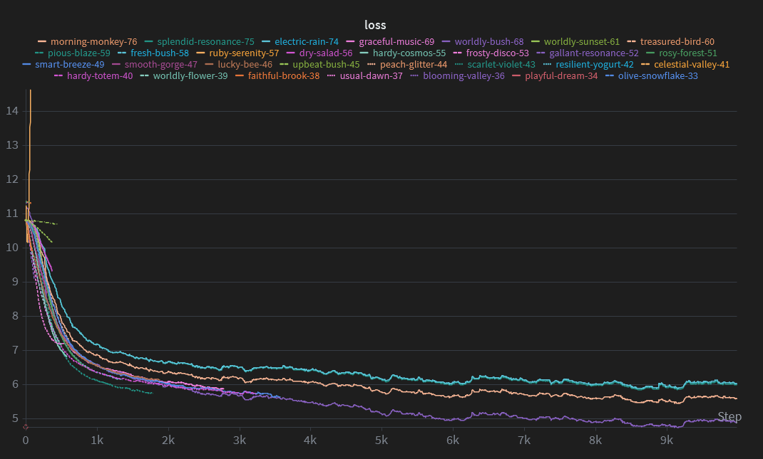
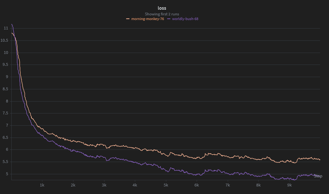Loss curves for ATLAS and the transformer baseline. Try to guess which is which!

Introduction

I saw this paper near the end of 2025 and thought it would be fun to implement. It was not, but I did learn a few new things while doing it.

ATLAS is a massive paper content-wise. The authors propose five different architectures, although they only go into detail for the last one (ATLAS). I am not unemployed enough to implement all five, so I have limited myself to just the ATLAS architecture.

The main contribution of this paper is the idea of treating the state as its own neural network mapping keys to values and optimizing it over a set of tokens, rather than one at a time (Omega rule).

Background

Following Songlin Yang’s DeltaNet Explained (Part I), normally, in vanilla linear attention (removing the $\exp$), we have

\[o_i =\sum_{j=1}^i (q_i^\top k_j)v_j\]

Where $o_i \in \mathbb{R}^{d_\text{head}}$ is the output of attention for token $i$ and $q_i, k_j, v_j \in \mathbb{R}^{d_\text{head}}$ are the query, key, and value vectors.

If we keep a running sum of the outer products between all the values and keys and let $S_i = \sum_{j=1}^i v_k k_j^\top$, then we get

\[S_i q_i = (\sum_{j=1}^i v_k k_j^\top)q_i \newline = \sum_{j=1}^i v_k \underbrace{(k_j^\top q_i)}_\text{scalar} \newline = \sum_{j=1}^i (q_i^\top k_j)v_j = o_i\]

In normal attention, if we attempt to retrieve a value for a given key $k_t$, we have

\[\sum_{j=1}^i\frac{ \exp(k_t^\top k_j)}{\sum_{\ell=1}^i \exp(k_t^\top k_\ell)}v_j\]

Ideally, when $j \ne t$, the dot product between $k_t$ and $k_j$ will be relatively small and $v_j$ will not contribute much to the output. When $j=t$, $\exp(k_t^\top k_t) = \exp(||k_t||^2)$, which should be a relatively large number, so the output of attention will be $v_t$ plus some noise. Note that $k_t$ and $k_j$ do not need to be orthogonal for all $j \ne t$ in order for this to happen. Their dot product could be small or negative and it would still become squashed by the softmax relative to a large value.

In removing the $\exp$, we lose this property. Basically all the keys have to be orthogonal to avoid retrieval error, which means the amount the model can remember is limited by its head dim.

1. The Memory Module

The authors view attention as a learnable mapping function from keys to values. Instead of simply adding to a matrix-valued state, they propose to use a neural network that is trained to learn this mapping as the model goes through the sequence at test time.

\[v_\text{pred} = \mathcal{M}_t(k_t)\] \[\mathcal{L} = ||v_t - v_\text{pred}||_2^2\] \[\mathcal{M}_{t+1} = \mathcal{M}_t - \eta_t \nabla \mathcal{L}_\mathcal{M}\]

With this, we get

\[\mathcal{M}(k_j) \approx v_j\]

Which is similar to vanilla linear attention. This network is trained by treating all the other model parameters as hyperparmeters and just optimizing with respect to the parameters of the inner network. There is likely a way to use torch’s autograd for this, but I opted to just keep the size of the memory small (2 layers) and calculated the gradients manually. Unfortunately, this makes the code a bit messy as the weights and states aren’t abstracted inside of nn.Module objects and need to be individually updated.

The authors also propose to use Muon when training the internal memory by keeping track of the running average state $S_t$ and orthogonalizing the updates with newton-schulz.

def newtonschulz5(
    x: torch.Tensor,
    iterations: int = 5,
    coeffs: tuple[float] = (3.4445, -4.775, 2.0315),
    epsilon: float = 1e-5,
) -> torch.Tensor:
    x = x / (x.norm() + epsilon)

    for _ in range(iterations):
        x = (
            coeffs[0] * x
            + coeffs[1] * x @ x.T @ x
            + coeffs[2] * (x @ x.T) @ (x @ x.T) @ x
        )

    return x

1.1 Omega rule

---

Part of the contribution of ATLAS is Omega rule, which describes optimizing the loss over a window of tokens as opposed to online (last token only). Take for example the following sequence:

\[\text{Local man arrested for illegal possession of DDR5 RAM, sentenced to life in jail}\]

Suppose we are predicting the next token in the sequence with a transformer and we have a simple attention head that looks for context to nouns. This head’s query projection maps the embedding for $\text{jail}$ into some new vector. Then, for all the previous tokens in the sequence, the key projection maps them to vectors. Certain tokens, such as $\text{DDR5, RAM,}$ and $\text{local}$ will be mapped by the head’s projection matrices to a vector similar to the query produced for $\text{jail}$.

Because the keys for these tokens are similar to the query for $\text{jail}$, their values will have more weight in the output as the $q^\top k$ term in attention measures dot product similarity and is used to weight the corresponding values.

This would ideally help shift the embedding for $\text{jail}$ into a new vector that takes into account the context of $\text{DDR5 RAM}$ and other tokens.

---

If, instead of attention, we used a neural network memory $\mathcal{M}_t$ as described above, we would struggle with perfect mapping of keys to values due to the limited capacity of the network. Some would have to be compressed or forgotten entirely.

If we only optimize with respect to the last token in the sequence, the network will greedily memorize all the key-value mappings and likely overfit or entirely forget certain tokens.

However, if we sum the losses over a context window, the memory will be forced to learn a more general representation and will be less likely to completely erase information from past tokens in order to memorize new ones.

2. Polynomial Mapping

This was the hardest part of the paper for me to understand, and I likely did not implement it as the authors might have intended.

The purpose of the mapping seems simple. It expands the queries and keys in a mostly continuous way (as opposed to just appending random values to the vectors), which gives the memory MLP more mapping ability. It also approximates the $\exp$ function in regular attention, as $\phi(q)^\top \phi(k) \approx \exp(q^\top k)$.

However, I had some issues implementing it. The paper describes the polynomial mapping as follows:

\[\phi^*(x) = \begin{pmatrix} 1 \\ \frac{x}{\sqrt{1}} \\ \frac{x^\otimes 2}{\sqrt{2!}} \\ \frac{x^\otimes 3}{\sqrt{3!}} \\ \vdots \end{pmatrix}, \hspace{1cm} \phi_p(x) = x^{\otimes p}, \hspace{1cm} x^{\otimes p} = x \otimes x^{\otimes (p - 1)}\]

Unfortunately, this is very slow to calculate. I may have done something wrong, but my training loop with implementation was only getting a few hundred tokens per second. So, I instead used the method from PolySketchFormer, the paper that they cite for the polynomial kernels.

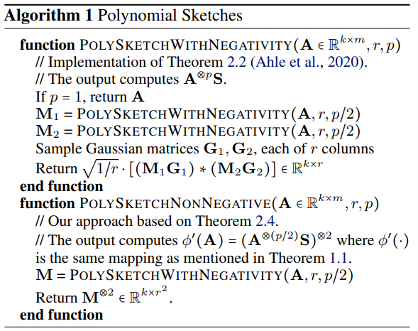
I have no idea why this works or if it is the method the ATLAS authors intended, but it performs much better than the naïve implementation, so I kept it.

def poly_sketch_with_negativity(
    A: torch.Tensor,
    r: int,
    p: int,
    deterministic: bool = False,
    gen: torch.Generator | None = None,
) -> torch.Tensor:
    if p == 1:
        return A
    gen = torch.Generator().manual_seed(42) if gen is None and deterministic else gen
    M_1 = poly_sketch_with_negativity(A, r, p // 2, gen)
    M_2 = poly_sketch_with_negativity(A, r, p // 2, gen)

    G_1, G_2 = (
        torch.randn(A.size()[:-2] + (A.size(-1), r), generator=gen).to(A.device),
        torch.randn(A.size()[:-2] + (A.size(-1), r), generator=gen).to(A.device),
    )
    return (1 / r) ** 0.5 * ((M_1 @ G_1) * (M_2 @ G_2))


def poly_sketch_non_negative(
    A: torch.Tensor, r: int, p: int, deterministic: bool = False
) -> torch.Tensor:
    M = poly_sketch_with_negativity(A, r, p // 2, deterministic=deterministic)

    M = torch.einsum("...i, ...j -> ...ij", M, M).squeeze(-1)
    res = torch.einsum("...i, ...j -> ...", M, M)
    return res

3. The Model Architecture

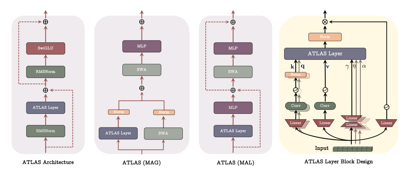
I was expecting the architecture to be super complex (see RWKV), but it was mostly transformer-like outside of the memory module. The only notable exception was the size 4 convolution layers following the $q, k, v$ projections. This was not too difficult to implement and just involved padding the $n-1$ positions to the left to prevent future tokens from leaking in:

class CausalConv1d(nn.Conv1d):
    def __init__(self, in_channels: int, out_channels: int, kernel_size: int):
        """Conv1d but with causal padding (kernel_size - 1)"""
        self.__padding = kernel_size - 1
        super().__init__(
            in_channels=in_channels,
            out_channels=out_channels,
            kernel_size=kernel_size,
            padding=self.__padding,
        )

    def forward(self, x: torch.Tensor) -> torch.Tensor:
        return super().forward(x)[..., : -self.__padding]

Interestingly, while I was doing some experiments, I found that increasing the size to greater than 4 seemed to make the model quite a bit better for only a slight tradeoff in performance. The parameter count did increase significantly, though, which is likely why the authors chose to fix the size at 4.

I also learned about gated MLPs, which are much simpler than I had expected. Instead of

\[y = \sigma(xW_1 + b_1)W_2 + b_2,\]

Gated MLPs use another layer without an activation and elementwise multiply:

\(y = (\text{Swish}_1(xW_1) \otimes (xV))W_2\) where \(\text{Swish}_\beta(x) = x \sigma (\beta x)\)

(see GLU Variants Improve Transformer).

Here is my implementation:

class SwiGLU(nn.Module):
    def __init__(
        self, in_size: int, hidden_size: int, out_size: int, beta: float = 1.0
    ):
        """SwiGLU as described in https://arxiv.org/abs/2002.05202"""
        super().__init__()
        self.in_size = in_size
        self.out_size = out_size
        self.beta = beta

        self.W = nn.Linear(in_size, hidden_size)
        self.V = nn.Linear(in_size, hidden_size)

        self.sigmoid = nn.Sigmoid()

        self.W2 = nn.Linear(hidden_size, out_size)

    def swish(self, x: torch.Tensor) -> torch.Tensor:
        return x * self.sigmoid(self.beta * x)

    def forward(self, x: torch.Tensor) -> torch.Tensor:
        return self.W2(self.swish(self.W(x)) * self.V(x))

4. Training

I started a total of 131 training runs between ATLAS and PolySketchFormer. Most of these only lasted a few steps before being restarted with different hyperparams. In the end, I settled with the following configuration:

Setting	Value
Optimizer	Muon (AdamW for non-square params)
lr	1e-3 (3e-4 for AdamW, cosine decay)
Warmup steps	200
Total batch size	16
Sequence length	512
Chunk size	64

And used the 170M parameter settings described in Appendix E of the paper.

When I first ran the training script, I was getting around 700 tokens/s. After a bit of messing around, I found that this was caused by two things.

The first was the polynomial kernel. I quickly fixed this by just using the implementation from PolySketchFormer. The second took me a little longer to notice. I assumed I had implemented something wrong and spent quite a bit of time isolating the components of the model and inspecting their runtimes. This led me to the Memory module, which seemed to be very slow, but only for large sequences. I tried increasing the chunk size from 4 to 64 and my tokens/s instantly went up to 7000, and came closer to 15000 after torch.compile.

I spent a lot of time tuning the hyperparams and eventually got the loss down to about 5.5 on fineweb-edu after 2.5 hours of training on my gpu.

I was curious to see how this compared to a transformer, and wrote a quick and barely-tuned implementation to test.

Not too surprisingly, it did much better. The transformer achieved a loss of around 4.9 in nearly half the time (it was the purple line in the first image).

Here are all my training runs visualized:

What I Learned & Thoughts

Surprisingly, learning about linear attention has been the most effective tool for me to understand why regular attention works. It is very easy to simply take the formula for granted or just plug the numbers into torch.nn.functional.scaled_dot_product_attention(), but reading all this material about linear variants and following along with the math on my whiteboard has given me much more confidence in my knowledge. I am still far from understanding everything, but attention no longer feels like a complete black box to me.

---

It seems to me that while linear attention-based architectures may become more prevalent in the future, transformers are still the best option for small models most of the time*.

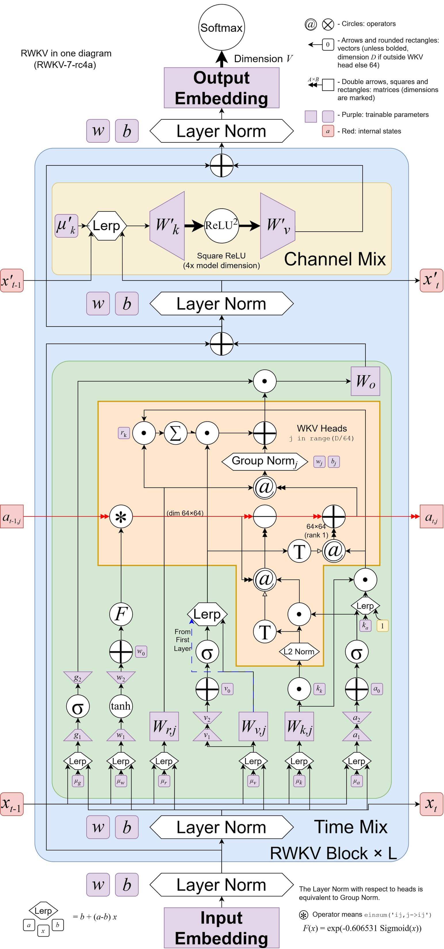
NOTE The exception to this is RWKV, which is shockingly good at small scale, and, in my experience, has performed much better than transformers for local training. If you can put up with the extremely confusing training repo and hopelessly complicated architecture, it is a very cool option to explore.

I can see how ATLAS would be beneficial for much longer sequence lengths where it becomes impossible to use the full quadratic attention. However, small models hardly benefit from million-token context windows and scaling batch size is often just as effective an option as sequence length. Long-context capability definitely has a lot of potential uses (eg. DNA sequnces, massive codebases), and if done correctly, I feel that linear attention models like ATLAS could be very helpful for training and inference efficiency.

Conclusion

ATLAS will not replace the transformer. I am almost entirely certain of this. It is too complex and too slow to be used widely for small models. However, the paper does not seem to be aimed toward small-scale use. It (or other linear attention models) might instead be implemented in the future by frontier labs focused on long-context tasks, though surely tons of modifications and custom CUDA kernels would be needed to make it a viable option.

Still, there has been a lot of promising recent research on these kinds of linear models, and I am optimistic to see what might come next.

References

Behrouz, A., Li, Z., Kacham, P., Daliri, M., Deng, Y., Zhong, P., Razaviyayn, M., & Mirrokni, V. (2025). ATLAS: Learning to Optimally Memorize the Context at Test Time. ArXiv.org. https://arxiv.org/abs/2505.23735

Kacham, P., Mirrokni, V., & Zhong, P. (2023). PolySketchFormer: Fast Transformers via Sketching Polynomial Kernels. ArXiv.org. https://arxiv.org/abs/2310.01655

Shazeer, N. (2020). GLU Variants Improve Transformer. ArXiv:2002.05202 [Cs, Stat]. https://arxiv.org/abs/2002.05202

Yang, S. (2024). DeltaNet Explained (Part I) | Songlin Yang. GitHub Pages. https://sustcsonglin.github.io/blog/2024/deltanet-1/