Java MNIST from scratch
MNIST Classifier from scratch in Java
[Link to the full code]
Background
Of all the possible programming languages to use for training a handwritten digit classifer, Java would not be my first choice. Although, to be fair, it wouldn’t be my first choice for doing anything else, either.
CS210 at my college is taught entirely in Java. I decided to make this as a first java project to learn the syntax. Sometimes it can be good to stray away from the warmth and comfort of abstraction that torch’s autograd so generously provides and do manual derivatives like a neanderthal.
Overview
The Matrix and Vec classes
Not wanting to dive too deep into optimized matmul kernels, I opted for an object-oriented approach, using a Vec class with a dot() method and a Matrix class made up of Vecs.
The Vec class
1
2
3
4
5
6
7
8
9
10
11
12
13
14
15
16
17
18
19
20
21
22
23
24
25
26
27
public class Vec {
    // store an array of doubles
    public double[] data;

    public Vec(double[] data) {
        // init with preset data
        this.data = data;
    }

    public Vec(int length) {
        // zero-init if given length
        this.data = new double[length];
    }

    public double dot(Vec other) {
        assert this.data.length == other.data.length : "vectors must be of same length for dot product";
        double out = 0.0;

        for (int i = 0; i < this.data.length; i++) {
            out += this.data[i] * other.data[i];
        }
        return out;
    }

    // other methods
}
The Matrix class
1
2
3
4
5
6
7
8
9
10
11
12
13
14
15
16
17
18
19
20
21
22
23
24
25
26
27
28
29
30
31
32
33
34
35
36
37
38
39
40
41
42
43
44
45
46
47
48
49
50
51
52
53
54
55
56
57
58
59
60
61
62
63
64
65
66
67
68
69
70
71
72
73
74
75
76
77
78
79
80
81
82
83
84
85
86
87
public class Matrix {
    // random for _rand function
    Random random = new Random();
    // need to store a list of values and their shape
    public Vec[] data;
    public int[] shape;

    public Matrix(Vec[] data) {
        // if given an array of vectors, use them as data and their lengths as shape
        this.data = data;
        this.shape = new int[] { data.length, data[0].data.length };
    }

    public Matrix(int rows, int cols) {
        // if given shape, zero-init
        this.data = new Vec[rows];
        for (int i = 0; i < rows; i++) {
            this.data[i] = new Vec(cols);
        }
        this.shape = new int[] { rows, cols };
    }

    public int numel() {
        // count number of elements in the matrix
        return this.shape[0] * this.shape[1];
    }

    public double[] flatten() {
        // squish into 1 dimension
        double[] out = new double[this.shape[0] * this.shape[1]];
        for (int i = 0; i < this.shape[0]; i++) {
            for (int j = 0; j < this.shape[1]; j++) {
                out[i * this.shape[1] + j] = this.data[i].data[j];
            }
        }
        return out;
    }

    public Matrix view(int rows, int cols) {
        // try to reconstruct (m x n) matrix from (mn) data
        Matrix out = new Matrix(rows, cols);

        double[] flattened = this.flatten();

        for (int i = 0; i < rows; i++) {
            for (int j = 0; j < cols; j++) {
                out.data[i].data[j] = flattened[i * (cols - 1) + j];
            }
        }

        return out;
    }

    public Matrix transpose() {
        // loop through rows and cols and flip flop
        Matrix out = new Matrix(this.shape[1], this.shape[0]);
        for (int i = 0; i < this.shape[0]; i++) {
            for (int j = 0; j < this.shape[1]; j++) {
                out.data[j].data[i] = this.data[i].data[j];
            }
        }

        return out;
    }

    public Matrix matmul(Matrix other) {
        // if A is (h x i) and B is (j x k), make sure i==j
        assert this.shape[1] == other.shape[0] : "inner shapes must match for matmul";
        // out is (h x k)
        Matrix out = new Matrix(this.shape[0], other.shape[1]);
        // dot product-ing the rows of A with the columns of B is the same as rows of A
        // with rows of B.T
        Matrix transposed = other.transpose();

        // do dot products
        for (int i = 0; i < this.shape[0]; i++) {
            for (int j = 0; j < other.shape[1]; j++) {
                out.data[i].data[j] = this.data[i].dot(transposed.data[j]);
            }
        }

        return out;
    }

    // other methods

}
Training Details
I use a 2-layer MLP (784 -> hiddenDim -> 10) as the model, which predicts the one-hot vector representing the label using $\text{MSE}$ loss.
e.g.
\[\text{target} = \begin{bmatrix} 0 \\ 0 \\ \vdots \\ 1 \\ 0 \\ 0 \\ \end{bmatrix}\]Where the $n$ th (label) element of the vector is $1$ and all other elements are $0$.
Cross-entropy would be better, but much harder to implement in terms of tensor operations, since it requires indexing and broadcasting. Since MNIST is a relatively simple problem, I stuck with $\text{MSE}$ and a simple SGD optimizer.
Without any form of autograd, it was necessary to find the gradients manually. Luckily, for a two-layer MLP, this isn’t super hard.
As a little side note, I found that scaling the parameter values before training by dividing by $\sqrt{\text{fan in}}$ and multiplying by the tanh gain of $\frac{5}{3}$ was extremely helpful to the model’s performance. Accuracy jumped from around $0.6$ to $0.9$ just with this change.
Manual Backprop
Since I’ve only taken up to Calculus III at this point, I don’t really have a full understanding of calculus with matrices or even just linear algebra. However, considering operations done to the individual elements of each intermediate result matrix is usually enough.
To find the gradient of each intermediate result matrix, we start with the loss and work backwards.
With $\text{MSE}$, the loss is defined as
\[\mathcal{L} = \frac{1}{N} \sum_{i=1}^N \left(y_i - \hat{y}_i\right)^2\]Where $y_i$ is the label (in this case our one-hot vector from earlier) and \(\hat{y}_i = f_{\theta}(x)\)
is the output of the model $f_{\theta}$ with input $x$ and parameters $\theta$.
$\text{sum}$
The loss can be split up into multiple operations. The last intermediate tensor before the loss is the sum \(\text{sum} = \sum_{i=1}^n \left(y_i - \hat{y}_i\right)^2\)
Loss can be thought of as a function of this sum.
\[\mathcal{L} = \frac{1}{N} \cdot \text{sum}\]Since $\frac{1}{N}$ is a constant,
\[\frac{\partial \mathcal{L}}{\partial \text{ sum}} = \frac{1}{N}\]$\text{diff}^2$
The sum can also be decomposed.
If the squared difference vector, \(\left(y_i-\hat{y}_i\right)^2,\)
Has $10$ elements,
\[\text{diff}^2 = \begin{bmatrix} x_1 \\ x_2 \\ x_3 \\ \vdots \\ x_{10} \end{bmatrix}\]Then, the sum \(\sum_{i=1}^{n} \text{diff}^2 = x_1 + x_2 + x_3 + \dots + x_{10}.\)
We can see that \(\frac{\partial \text{ sum}}{\partial x_1} = 1.\)
The same is true for all elements $x_n$ of $\text{diff}^2$. This means that
\[\frac{\partial \text{ sum}}{\partial \text{ diff}^2} = \begin{bmatrix} 1 \\ 1 \\ 1 \\ \vdots \\ 1 \end{bmatrix}\](Again, I don’t know if this is correct notation or anything but this is my thought process).
We can then use the chain rule to find $\frac{\partial \mathcal{L}}{\partial \text{ diff}^2}$.
\[\frac{\partial \mathcal{L}}{\partial \text{ diff}^2} = \frac{\partial \mathcal{L}}{\partial \text{ sum}} \cdot \frac{\partial \text{ sum}}{\partial \text{ diff}^2} = \boxed{\frac{1}{N} \cdot \begin{bmatrix} 1 \\ 1 \\ 1 \\ \vdots \\ 1 \end{bmatrix}}\]I combine the above two steps into one in the training code:
1
Matrix ddiff2 = new Matrix(diff2.shape[0], diff2.shape[1]).op(k -> k + 1. / diff2.numel());
The Matrix() constructor makes a new zero-filled matrix, in this case with shape $(1, N)$. I use op(), which applies an elementwise lambda function to the matrix, passing in k -> k = 1. / diff2.numel() to fill the matrix with $\frac{1}{N}$.
$\text{diff}$
The next intermediate result matrix is $\text{diff}$, a $(1, N)$ matrix.
\[\text{diff}^2(\text{diff}) = \text{diff}^2\]Pretty crazy. Taking the derivative is simple, though.
\[\frac{\partial \text{ diff}^2}{\partial \text{ diff}} = 2 \cdot \text{diff}\]Then, using the chain rule,
\[\frac{\partial \mathcal{L}}{\partial \text{ diff}} = \frac{\partial \mathcal{L}}{\partial \text{ diff}^2} \cdot \frac{\partial \text{ diff}^2}{\partial \text{ diff}} = \boxed{\frac{\partial \mathcal{L}}{\partial \text{ diff}^2} \cdot 2 \cdot \text{diff}}\]For the gradient $\nabla \text{diff}$, we just plug in the current value of diff.
1
Matrix ddiff = ddiff2.multiply(diff.op(k -> k * 2.));
Where multiply() is element-wise multiplication.
$\text{out}$
The intermediate result $\text{diff}$ is a function of the two matrices $\text{out}$ ($\hat{y}$, or the model prediction, from before) and $\text{y}$ (the labels). Since $y$ is not a function of any other matrices and is not a parameter, there is no need to find its gradient.
Note that \(\text{diff}(\text{out}, \text{y}) = y - \text{out}\)
So \(\frac{\partial \text{ diff}}{\partial \text{ out}} = -1\)
Which is the same for all elements of $\text{out}$.
Using the chain rule once again,
\[\frac{\partial \mathcal{L}}{\partial \text{ out}} = \frac{\partial \mathcal{L}}{\partial \text{ diff}} \cdot \frac{\partial \text{ diff}}{\partial \text{ out}} = \boxed{\frac{\partial \mathcal{L}}{\partial \text{ diff}} \cdot -1}\]Here is the code which implements this:
1
Matrix dout = ddiff.op(k -> -k);
$L_1$
The two layer MLP can be decomposed as follows.
$f_\theta(X; W_1, W_2, b) = \text{tanh}(X \times W_1 + b) \times W_2$
Let the intermediate result $L_1 = \text{tanh}(X \times W_1 + b)$. Then,
\[f_\theta(L_1, W_2) = L_1 \times W_2\]To find the derivatives, it is probably best to break down what happens in matrix multiplication.
Take the following example involving the matrices $A (i, k)$ and $B (k, j)$ which are multiplied to get $C (i, j)$.
\[C = A \times B = \begin{bmatrix} a_{11}b_{11} + a_{12}b_{21} + \dots + a_{1k}b_{k1} & a_{11}b_{12} + a_{12}b_{22} + \dots + a_{1k}b_{k2} & \dots & a_{11}b_{1j} + a_{12}b_{2j} + \dots + a_{1k}b_{kj} \\ \\ a_{21}b_{11} + a_{22}b_{21} + \dots + a_{2k}b_{k1} & a_{21}b_{12} + a_{22}b_{22} + \dots + a_{2k}b_{k2} & \dots & a_{21}b_{1j} + a_{22}b_{2j} + \dots + a_{2k}b_{kj} \\ \vdots & \vdots & \ddots & \vdots\\ a_{i1}b_{11} + a_{i2}b_{21} + \dots + a_{ik}b_{k1} & a_{i1}b_{12} + a_{i2}b_{22} + \dots + a_{ik}b_{k2} & \dots & a_{i1}b_{1j} + a_{i2}b_{2j} + \dots + a_{ik}b_{kj} \\ \end{bmatrix}\]What if we try to find the partial derivative of a random element of $C$, say $C_{32}$, with respect to $a_{31}$.
\[C_{32} = \sum_{n=1}^k a_{3n}b_{n2} = \underline{a_{31}}b_{12} + a_{32}b_{22} + a_{33}b_{32} + \dots + a_{3k}b_{k2}\] \[\frac{\partial C_{32}}{\partial a_{31}} = b_{12}\]In general,
\[C_{ij} \sum_{n=1}^k a_{in}b_{nj}.\]However, note that if we try to find the gradient of $C_{32}$ with respect to $a_{21}$, we get:
\[C_{32} = \sum_{n=1}^k a_{3n}b_{n2} = a_{31}b_{12} + a_{32}b_{22} + a_{33}b_{32} + \dots + a_{3k}b_{k2}\]in which $a_{21}$ is not included (since the row of $a$ does not correspond to the column of $b$). This means that \(\frac{\partial C_{32}}{\partial a_{21}} = 0\)
Therefore, the partial derivatives wrt $a$ are:
\(\frac{\partial C_{ij}}{\partial a_{pq}} = \begin{cases} b_{qj}, &\text{if } i=p, \\ 0 &\text{otherwise} \end{cases}\) and similarly for $b$, \(\frac{\partial C_{ij}}{\partial b_{pq}} = \begin{cases} a_{jq}, &\text{if } i=p, \\ 0 &\text{otherwise} \end{cases}\)
Using the chain rule and removing the unnecessary summation over $i$ because of the zeros,
\[\frac{\partial \mathcal{L}}{\partial a_{pq}} = \sum_i \sum_j \frac{\partial \mathcal{L}}{\partial C_{ij}} \frac{\partial C_{ij}}{\partial a_{pq}} = \sum_j \frac{\partial \mathcal{L}}{\partial C_{ij}} b_{qj} \implies \frac{\partial \mathcal{L}}{\partial C} \times B^\top\]The above is very complicated, and probably incorrect since I am bad at math. Hence, I propose a much simpler method for finding the gradients, which is to look at the shapes of the matrices. We know that the shape of each gradient must be the same as the shape of its corresponding parameter. Using this knowledge and keeping in mind that the derivative should have something to do with matrix multiplication and transposes, we can find the formula for the gradient just by analyzing the input and output shapes.
Take for example our current case of $\text{out} = L_1 \times W_2$.
Because of the chain rule, we can assume that the partial derivative of $\text{out}$ with respect to $L_1$ must be multiplied by the gradient of the loss with respect to $\text{out}$.
$\nabla \text{out}$ is of shape $(1, 10)$
$W_2$ is of shape $(d_{\text{hidden}}, 10)$
And we need a gradient for $L_1$ of shape $(1, d_{\text{hidden}})$.
The only logical combination of $\nabla \text{out}$ and $W_2$ that produces an output of shape $(1, d_{\text{hidden}})$ is \(\boxed{\nabla \text{out} \times W_2^\top}\)
And it turns out, this is the same result as before. Nice.
1
Matrix dl1 = dout.matmul(w2.transpose());
$W_2$
We can use a similar method to find the gradient of the loss with respect to $W_2$.
We know:
$\nabla \text{out}$ is of shape $(1, 10)$
$L_1$ is of shape $(1, d_{\text{hidden}})$
and we need a gradient of shape $(d_{\text{hidden}}, 10)$
Therefore, $W_2$’s gradient is probably
\[\boxed{L_1^\top \times \nabla \text{out}}\]1
Matrix dw2 = l1.transpose().matmul(dout);
$L_{1b}$
I will use $L_{1b}$ to refer to the intermediate result $X \times W_1 + b$. Therefore, $L_1(L_{1b}) = \text{tanh}(L_{1b})$.
Since $L_{1b}$ and $L_1$ are the same shape and $\tanh$ is applied elementwise, finding the gradient is fairly simple.
\[\text{tanh}(x) = \frac{\text{sinh}(x)}{\text{cosh}(x)} = \frac{e^{2x}-1}{e^{2x}+1}\]\(\frac{d}{dx}\text{tanh}(x) = \frac{d}{dx}\left[\frac{e^{2x}-1}{e^{2x}+1}\right] = \frac{(2e^{2x})(e^{2x}+1) - (e^{2x}-1)(2e^{2x})}{\left(e^{2x}+1\right)^2} = \frac{4e^{2x}}{\left(e^{2x}+1\right)^2}\) \(\frac{\partial \mathcal{L}}{\partial L_{1b}} = \frac{\partial \mathcal{L}}{\partial L_1} \frac{\partial L_1}{\partial L_{1b}} = \boxed{\frac{\partial \mathcal{L}}{\partial L_1}\cdot \frac{4e^{2L_{1b}}}{\left(e^{2L_{1b}} + 1\right)^2}}\)
And here is the implementation, where tanhDerivative is a utility function for the derivative of $\text{tanh}$ applied elementwise.
1
Matrix dl1biased = dl1.multiply(l1biased.tanhDerivative());
$b$
My variable naming is a little bit cursed since I didn’t add bias until later, but $L_{1b}$ can be defined as
\[L_{1b}(L_{1\text{preact}}, b) = L_{1\text{preact}} + b\]Therefore,
\[\frac{\partial L_{1b}}{\partial b} = 1\]and
\[\frac{\partial \mathcal{L}}{\partial b} = \frac{\partial \mathcal{L}}{\partial L_{1b}} \frac{\partial L_{1b}}{\partial b} = \boxed{ \frac{\partial \mathcal{L}}{\partial L_{1b}} }.\]1
Matrix db = dl1biased;
$L_{1\text{preact}}$
$L_{1\text{preact}}$ is the input multiplied by the first hidden layer, and is added together with the bias $b$. Much like the bias, its partial derivative with respect to $L_1$ is $1$. This means its gradient is also the same:
1
Matrix dl1preact = dl1biased;
$W_1$
The first weight matrix is multiplied with the input to get $L_{1\text{preact}}$. Using the shape analysis method once again to find the gradient, we see the following:
$\nabla L_{1\text{preact}}$ is of shape $(1, d_{\text{hidden}})$
$X$ is of shape $(1, 784)$
And we need a gradient of shape $(784, d_{\text{hidden}})$ for $W_1$.
The most sensible operation to get a matrix of this shape would be
\[\nabla W_1 = \boxed{X^\top \times \nabla L_{1\text{preact}}}\]Therefore,
1
Matrix dw1 = x.transpose().matmul(dl1preact);
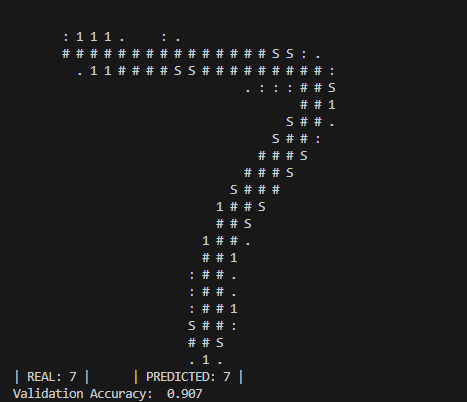
Testing the model
A handwritten digit classifier isn’t very useful if you can’t at least try it out yourself. To do this, I made a quick drawing screen using java swing that showed the model’s prediction of the current image.
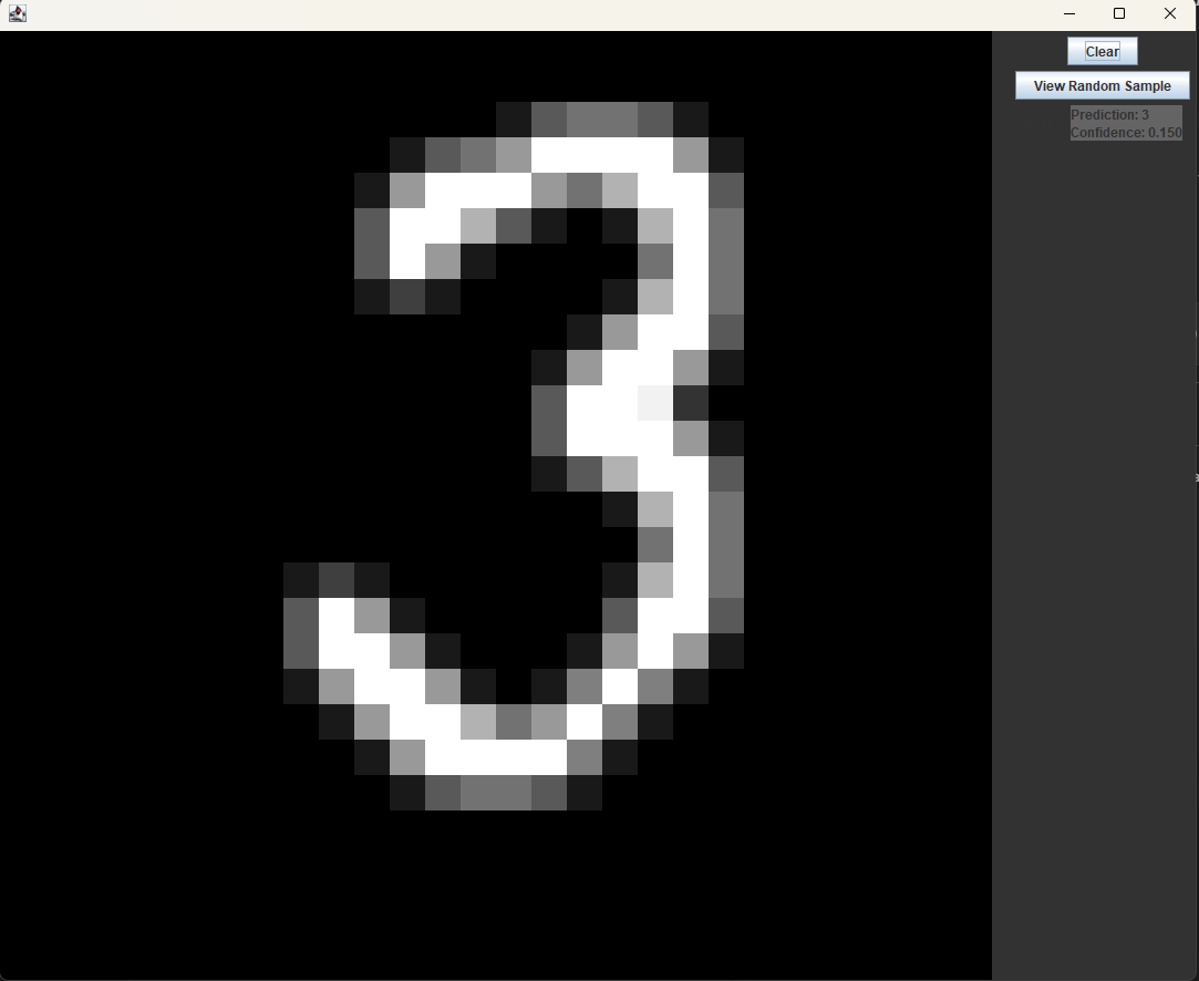
The app itself worked (mostly) fine, but the model’s accuracy was terrible. It was scoring 93% on the test data, but for some reason could barely recognize any of the digits I was drawing. The model was consistently wrong, for no apparent reason.
I spent multiple days debugging this, printing out the image buffer to look for incorrect formatting, checking for unexpected changes in the weights, and improving the model, but found nothing.
My handwriting couldn’t be that far out of the training distribution, could it?
In the time I spent contemplating the issue, I came across a demo of a model online with a reported 98% accuracy. I tested it out and found that it was almost never wrong, even when I purposefully tried to make the digits less legible.
I then noticed that there was an option to disable cropping on the images. I tried turning this option off, and whenever I drew a digit slightly away from the center of the screen, the accuracy went down significantly. Interesting.
A quick look at some of the images from the dataset revealed that they were all almost perfectly centered in the frame, meaning that even a slight shift in any direction would likely ruin the effectiveness of any model trained on them without data augmentation.
Rather than making the model more robust by training it on random translations of the images in the training data, I decided to fix this problem by implementing my own cropping algorithm. Every update in the GUI app, before the image buffer is sent to the model for classification, it is shifted so that there is equal distance right, left, above, and below the filled in pixels. This greatly improved the accuracy when testing and made the model finally usable.
Conclusion
This project reminded me of how much is truly abstracted behind big libraries like torch. Obviously, this is a necessary abstraction. Nobody wants to manually backpropagate through a $32$-layer transformer. If everyone had to write all their code from scratch in cuda, research would take forever.
Still, though, I think it is important not to take these tools for granted, and to take a step back every once in a while to appreciate all that is going on under the hood. While I could have done all this in just a few lines of python, I feel that taking the time to re-learn and better understand what I am doing is something much more valuable.