Tokenization and Training Improvements

Tokenization and Training Improvements

[Link to full code]

Introduction

There have been quite a few papers published recently that I have been wanting to implement, but have not yet had the time. These are mostly optimizations and enhancements to the transformer (DeepSeek mHC, Engram, Attention Residuals, XSA, etc).

I have also been interested in tokenization and whether a model with a smaller vocabulary could achieve performance similar to that of a larger model with less training time. Given that the embedding and output projection tend to make up a significant fraction of the parameters in smaller models, it seems possible that allocating more parameters in the interior of the model would allow it to learn more complex patterns in text with the same compute as opposed to simply driving down the probabilities of uncommon tokens in the projection.

Tokenization

Before looking at any resources, I attempted to create my own tokenizer using a greedy strategy:

# make string to int and int to string maps
N_VOCAB = 10000
stoi = {chr(i):i for i in range(256)}
itos = {i:chr(i) for i in range(256)}

def tokenize(text: str) -> list[int]:
    # Greedy tokenization strategy: keep a buffer 
    # and add until no longer in vocab
    out = []
    buffer = ""
    for char in text:
        if buffer in vocab and buffer + char not in vocab:
            out.append(vocab[buffer])
            buffer = ""
        buffer += char
    
    out.append(stoi[buffer])

tokens = tokenize(input_text)
    
while (vocab_size := len(stoi)) < N_VOCAB:
    # keep merging most frequent pair and retokenize
    tokens = tokenize(input_text)
    frequencies = {}
    
    for t1, t2 in zip(tokens, tokens[1:]):
        pair = t1 + t2
        freq = frequencies[pair]
        frequencies[pair] = freq + 1 if freq is not None else 1

    merge = max(frequencies)

    vocab_size = len(stoi)
    stoi[merge] = vocab_size
    itos[vocab_size] = merge

This approach was unfortunately very slow and inefficient with vocabulary (for SANDWICH to be encoded as a single token, there would have to be a SANDWIC token due to greedy encoding).

So, I decided to look into Byte-Pair Encoding (BPE). The idea is fairly simple and somewhat similar to what I was attempting to do before.

We start with a set of bytes (utf8-encoded text):

70 111 114 116 110 105 116 101 32 66 97 108 108 115 ...

And a vocabulary that starts by simply mapping each byte to itself:

{
    1 : 1,
    2 : 2,
    ...
    255 : 255,
}

For each pair of tokens, eg.

(70, 111), (111, 114), (114, 116) ...

We count the frequencies of each in the text:

{
    (70, 111) : 1,
    (111, 114) : 3,
    (93, 84) : 7,
    ...
}

And then add the most common frequency pair to the vocabulary with the next token index.

{
    1 : 1,
    2 : 2,
    ...
    255 : 255,
    256 : (93, 84),
}

Keep doing this until the vocabulary is the desired size. For inference, simply perform all these merges in the order they were found in training.

I decided to implement this in Java. Training was not much of a problem as I could simply limit the amount of input data, but encoding the entire dataset afterwards was much too slow. My first implementation was the following:

public List<Integer> encode(ByteBuffer input) {
    List<Integer> tokens = new ArrayList<>();

    // O(n)
    while (input.hasRemaining()) {
        tokens.add((int) (input.get() & 0xff));
    }

    // ~O(n^2)
    while (true) {
        // O(n)
        Set<TokenPair> merges = new HashSet<>();
        for (int i = 1; i < tokens.size(); i++) {
            TokenPair merge = new TokenPair(tokens.get(i - 1), tokens.get(i));
            if (this.vocab.containsValue(merge))
                merges.add(merge);
        }

        // O(n)
        Iterator<TokenPair> iter = merges.iterator();
        TokenPair minMerge = null;
        int minIdx = this.vocabSize;
        boolean hasMerge = false;
        while (iter.hasNext()) {
            TokenPair merge = iter.next();

            if (this.vocab.containsValue(merge)) {
                int idx = this.vocab.getKey(merge);

                if (idx > 255) {
                    if (idx < minIdx) {
                        minMerge = merge;
                        minIdx = idx;
                    }

                    hasMerge = true;
                }

            }
        }

        if (!hasMerge || minMerge == null)
            break;
        
        ArrayList<Integer> newTokens = new ArrayList<>(tokens.size());
        Iterator<Integer> tokensIter = tokens.iterator();
        
        // O(n)
        int last = tokensIter.next();
        while (tokensIter.hasNext()) {
            int current = tokensIter.next();

            TokenPair combined = new TokenPair(last, current);

            if (combined.equals(minMerge)) {
                newTokens.add(this.vocab.getKey(combined));
                if (tokensIter.hasNext())
                    current = tokensIter.next();
            } else {
                newTokens.add(last);
                if (!tokensIter.hasNext())
                    newTokens.add(current);
            }

            last = current;
        }

        tokens = newTokens;
    }

    return tokens;
}

This implementation runs in approximately $\mathcal{O}(mn)$ time with $m$ merges and $n$ bytes, which doesn’t seem terrible, but it achieves only a measly 9000 tok/s. This can be improved.

A bit of profiling revealed that adding to the merges was taking a decent amount of time each loop (0.8ms). Increasing the default HashSet capacity improved this to 0.4ms. I also sped up adding the initial tokens by setting the default capacity of the tokens ArrayList.

I also got a 40x speedup by simply reducing the chunk size to 16 from 16384 since the algorithm runs in $\mathcal{O}(mn) \approx O(n^2)$ time. I could likely reduce this even further, but I am afraid of small chunks decreasing the quality. (With chunk size 16 I get ~400k tok/s).

Unfortunately, this was not enough. I decided to implement a word split regex and token lookup.

We can store the string values of all the tokens in our vocabulary for lookup as follows:

private void buildCache() {
    for (int i: this.vocab.keySet()) {
        this.tokenCache.put(this.toString(this.vocab.getValue(i)), i);
    }
}

This results in something like:

{
    " hello" : 2342,
    " py" : 1764,
    ...
    "USER: " : 1934,
}

If we split the string using a regex:

public class Tokenizer {
    // ...

    private Pattern pretokRegex = Pattern.compile("\\s+");


    // ...

    public List<Integer> encode(String input) {
        String[] pretokens = this.pretokRegex.split(input);
        List<Integer> tokens = new ArrayList<>(pretokens.length * 2); // there will probably be about 2 tokens per word
        
        for (String pretoken: pretokens) {
            if (this.tokenCache.containsKey(pretoken)) {
                tokens.add(this.tokenCache.get(pretoken));
            } else {
                tokens.addAll(this.encode(StandardCharsets.UTF_8.encode(pretoken)));
            }
        }
        return tokens;
    }
}

Then, for most tokens, we can just index into the cache and only do BPE for the ones that can’t be indexed.

This resulted in about 750k tok/s.

I noticed that the tokenizer was wasting a significant number of tokens on slight variations of strings, eg

["python", "python\n", "python\r\n", "python\n\n" ...]

So I made the pre-tokenization a bit stricter by disallowing special characters entirely in tokens. With an improved regex, I was able to get inference speeds of about 1M tok/s, which I used to tokenize about half of fineweb-edu.

Training

I made a quick vanilla transformer baseline with RoPE and SwiGLU to test the tokenizer on. The rest of the architecture is similar to the 120M GPT-2, aside from a 32k vocab size.

The smaller output projection led to a significant speedup over the 50304 baseline. Since most of the compute is spent on the projection, nearly halving the vocab size doubled my tok/s while training from ~16k to ~33k. After a bit of tuning, I was able to achieve a train loss of 2.85 on fineweb with just three hours of training on my GPU. Directly comparing the loss to GPT-2, this is nearly on par with the much larger (700M-1.5B) variants.

This is not a fair comparison, though.

Comparing models across tokenizers

Cross entropy measures loss per token and does not take into account the actual length of a sequence in characters.

For example, given the following sequence with assigned probabilities per token:

\[\underbrace{\text{[You]}}_{0.5} \underbrace{\text{[ should]}}_{0.4} \underbrace{\text{[ rewrite]}}_{0.3} \underbrace{\text{[ that]}}_{0.6} \underbrace{\text{[ in]}}_{0.8} \underbrace{\text{[ rust]}}_{0.9}\]

The cross-entropy loss is

\[\frac{1}{6} \left(-\log(0.5) -\log(0.4) - … - \log(0.9) \right) \approx 0.608 \text{ nats}\]

And the probability of the entire sequence as assigned by the model is

\[0.5 \times 0.4 \times 0.3 \times … \times 0.9 = 0.02592\]

However, if we have a less efficient tokenizer:

\[\underbrace{\text{[You]}}_{0.5} \underbrace{\text{[ sho]}}_{0.4} \underbrace{\text{[uld]}}_{0.7} \underbrace{\text{[ re]}}_{0.3} \underbrace{\text{[write]}}_{0.5} \underbrace{\text{[ that]}}_{0.6} \underbrace{\text{[ in]}}_{0.8} \underbrace{\text{[ r]}}_{0.9} \underbrace{\text{[ust]}}_{0.8}\]

The cross-entropy loss is:

\[\frac{1}{9} \left(-\log(0.5) -\log(0.4) -\log(0.7) - … - \log(0.8) \right) \approx 0.238 \text{ nats}\]

Which is much better than the first example, but the probability of the sequence as a whole is:

\[0.5 \times 0.4 \times 0.7 \times … \times 0.8 = 0.0072576\]

Which is much lower than before.

Clearly, the tokenizer has a large influence on the meaning of loss.

---

To compare models across tokenizers, the most commonly used metric is BPB (Bits Per Byte), which adjusts the per-token loss based on the number of characters per token.

\[\text{BPB} = \overbrace{\frac{\text{nats}}{\text{token}}}^{\text{per-token CE loss}} \times \frac{\text{tokens}}{\text{char (byte)}} \times \frac{\text{bits}}{\text{nat}}\]

Here is a Python pseudocode example:

def calc_bpb(logits: torch.Tensor, targets: torch.Tensor, enc: Tokenizer) -> float:
    """
    Estimates the BPB for the model given:
    logits:  (L, V)
    targets: (L)
    """
    # nats/token
    loss_sum = F.cross_entropy(logits.view(-1, logits.size(-1)), targets.view(-1), reduction="sum").item()

    # bytes/token
    bytes_sum = torch.Tensor([len(enc.decode([tok])) for tok in targets]).sum().item()

    return (loss_sum / bytes_sum) / math.log(2)

Testing this on our examples from before, we get:

\[\text{BPB}_\text{first} = \left(\frac{-\log(0.5) -\log(0.4) - … -\log(0.9)}{3 + 7 + … + 5 } \right) / \log(2) \approx 0.074 \text{ bits/byte}\]

And

\[\text{BPB}_\text{second} = \left(\frac{-\log(0.5) -\log(0.4) - … -\log(0.9)}{3 + 4 + … + 3 } \right) / \log(2) \approx 0.099 \text{ bits/byte}\]

Showing that the first model is indeed better. While we could just compare the probabilities assigned to a fixed sequence, doing so would require calculating the ratio of probabilities assigned by different models using numerical stability tricks with logs and exponentials, making it only possible to compare two models relative to each other at once.

Attention Residuals

I attempted to implement attention residuals first. The premise is mostly simple: instead of taking in only the output of the layer before it, each layer can now selectively access any of the previous hidden states from the model using an attention-like mechanism with its own learnable weight.

Instead of the normal

\[h_{n+1} = h_n + \text{Layer}(\text{norm}(h_n))\]

We have

\[h_{n+1} = h_n + \text{Layer}(\text{norm}(\text{Attention}(h_1, h_2 + … + h_n; q_\text{attn, n})))\]

I followed the implementation described in the paper, but the overhead was relatively large at the 160M model size, and ultimately underperformed the baseline on loss by time. I suspect the gains are only noticeable in larger-scale training, though it is entirely possible I have implemented the paper incorrectly.

XSA (Exclusive Self-Attention)

I next implemented XSA. The author of this paper noticed that the dot product similarity $q_i^\top k_j$ tends to be very large in attention when $i=j$ (tokens like to attend to themselves).

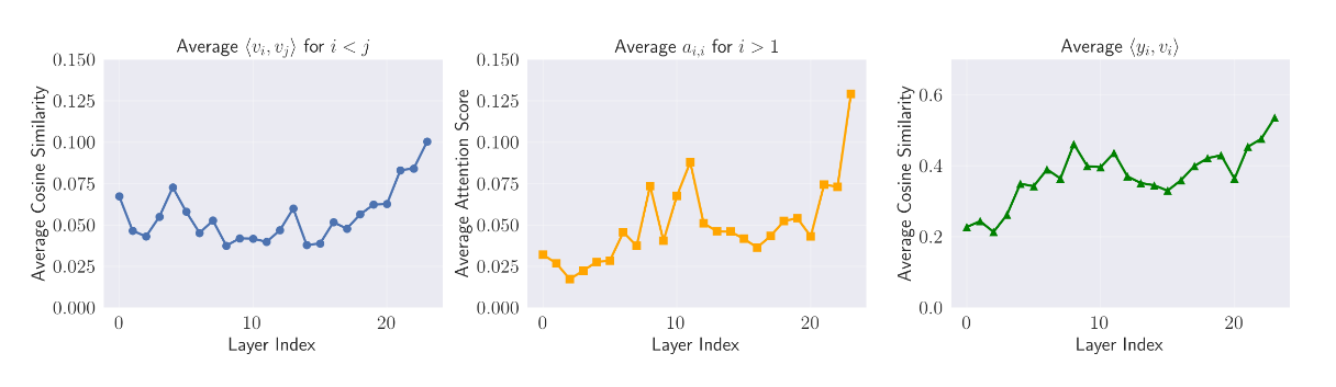
(From XSA Paper)

In order to remedy this, the paper proposes to “remove” the current value from the attention output by subtracting its projection onto the output.

\[z_i = y_i - \frac{y_i^\top v_i}{||v_i||_2^2}v_i\]

In theory, this should force the model to use attention to model more meaningful relationships between tokens.

However, it also fails to beat the baseline in wall-clock time.

Deepseek Engram

The Engram paper by DeepSeek proposes a way to add sparse parameters to a model in the form of n-gram embeddings. Since creating embeddings for all possible bi-grams and tri-grams is impossible, the authors use hashing and a large embedding table.

Engram uses multiple hash heads, each using their own hash function to map bigrams and trigrams to locations in the embedding table. These retrieved embeddings are concatenated, projected to $d_\text{model}$, and sent through a convolution layer before being selectively accessed via a projection weight.

\[([x_1, x_2]) \rightarrow \mathcal{H}_1, \mathcal{H}_2, …, \mathcal{H}_k \rightarrow \begin{bmatrix} 17 \\ 32 \\ 9 \\ 14 \\ \vdots \\ 6 \end{bmatrix} \rightarrow \text{ Embedding} \rightarrow \begin{bmatrix} 0.2 & 0.9 & -0.8 & … & 0.4 \\ 0.3 & -1.2 & 0.1 & … & 0.6 \\ \vdots & \vdots & \vdots & \vdots & \vdots \\ -0.7 & 0.5 & 0.2 & … & -0.3 \\ \end{bmatrix} \rightarrow \text{ concat}\]

I tried to tune engram to the best of my ability, but still was not able to get results better than the baseline. I think this again has to do with model scale. The template provided by DeepSeek uses quite a large model by default (~1B params not including engram) and doesn’t even include the full training code for comparison to a baseline, which leads me to believe that engram is simply not effective at smaller scales (much like MoE).

---

After some final tuning, I did a 20-hour pretraining run on fineweb with the following hyperparams:

Setting	Value
Optimizer	Muon (AdamW for non-square params)
lr	1e-2 (constant with linear warmup and cooldown)
Warmup steps	200
Micro batch size	16
Grad accum steps	16
Sequence length	512
Vocab size	32768

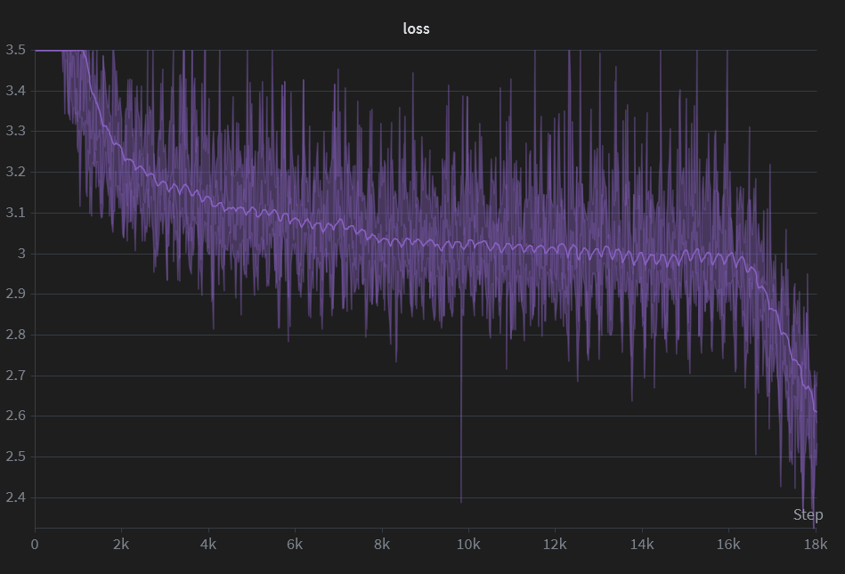
This resulted in a final loss of about 2.6 and BPB of about 1.06. This is slightly worse than the nanochat baseline of 0.97 trained on 1.1B tokens. I am unsure whether this is because of the lower vocab size of my model or other architectural/training improvements in nanochat that I have not yet implemented. Looking at nanochat, I see that Karpathy tuned the cooldown to be 40% of the total training time (much longer than my 10%), which could account for the difference, but I don’t want to spend another 20 hours waiting for my model to train and am happy with this result.

I then finetuned the model on a question/response coding dataset (glaive code assistant on huggingface). I have used this dataset in the past, and like the results it tends to give for small models, though it might not be wise to use it in serious, larger-scale SFT. The data is mostly comprised of question/answer exchanges related to Python.

Here is a mildly cherry-picked sample from the trained model:

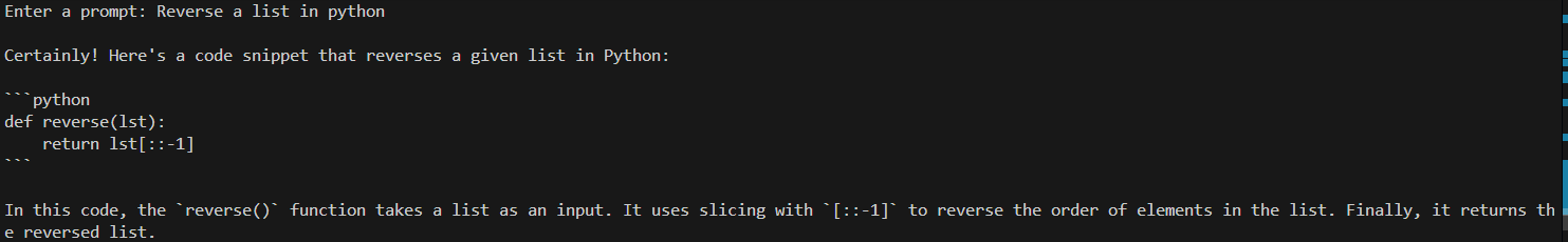
However, the model is a little bit deep-fried and outputs gibberish for anything even slightly out-of-distribution.

Reflections & What I Learned

There are a lot of things going on under the hood in LLM training that can be easy to overlook and terribly hard to debug. It took me nearly two weeks to realize that I had forgotten to call optim.zero_grad() in my training loop because the gradient clipping kept everything from breaking too visibly. There are probably still countless issues with the code in its current state that I will never know about. But I feel that with practice, I am getting better at guessing what is causing problems and knowing how to fix things.

---

Tokenizers are actually much less complex than I had expected in certain ways. Breaking down a string into tokens always seemed like a very difficult task to me, but the BPE approach of building up pair-by-pair is really quite simple.

While my initial hypothesis that shrinking the vocab size of a model would speed up training seems to be proven false, I still believe that there are gains to be made, especially in tokenization efficiency. While it is a pain to train a new tokenizer every time we want to train a new model, doing so can save a decent amount of compute, especially on datasets where the GPT-2 tokenizer is less efficient.

In the future, I might use something like rustbpe if I find myself needing a better domain-specific tokenizer. If you value your sanity, please do not write your own in Java.

References

Cheng, X., Zeng, W., Dai, D., Chen, Q., Wang, B., Xie, Z., Huang, K., Yu, X., Hao, Z., Li, Y., Zhang, H., Zhang, H., Zhao, D., & Liang, W. (2026). Conditional Memory via Scalable Lookup: A New Axis of Sparsity for Large Language Models. ArXiv.org. https://arxiv.org/abs/2601.07372

Karpathy, A. (2025). GitHub - karpathy/nanochat: The best ChatGPT that $100 can buy. GitHub. https://github.com/karpathy/nanochat

Karpathy, A. (2024, February 20). Let’s build the GPT Tokenizer. www.youtube.com. https://www.youtube.com/watch?v=zduSFxRajkE

patel, dip. (2025, October 16). Bits-per-Byte (BPB): a tokenizer-agnostic way to measure LLMs. Medium. https://medium.com/@dip.patel.ict/bits-per-byte-bpb-a-tokenizer-agnostic-way-to-measure-llms-25dfed3f41af

Shazeer, N. (2020). GLU Variants Improve Transformer. ArXiv:2002.05202 [Cs, Stat]. https://arxiv.org/abs/2002.05202

Su, J., Lu, Y., Pan, S.-F., Wen, B., & Liu, Y. (2021). RoFormer: Enhanced Transformer with Rotary Position Embedding. https://doi.org/10.48550/arxiv.2104.09864

Team, K., Chen, G., Zhang, Y., Su, J., Xu, W., Pan, S., Wang, Y., Wang, Y., Chen, G., Yin, B., Chen, Y., Yan, J., Wei, M., Zhang, Y., Meng, F., Hong, C., Xie, X., Liu, S., Lu, E., & Tai, Y. (2026). Attention Residuals. ArXiv.org. https://arxiv.org/abs/2603.15031

Zhai, S. (2026). Exclusive Self Attention. ArXiv.org. https://arxiv.org/abs/2603.09078