Flow Matching and Image Generation

Flow Matching and Image Generation

[Link to full code]

Introduction

Images are hard. Very hard.

I have spent the last ~2 years working almost exclusively on text-based models and NLP. I often take for granted the simplicity of the GPT-style architecture and training setup.

I assumed diffusion would be relatively easy. A few convolution layers stacked on top of one another, maybe with some residuals.

I watched videos, took notes, and felt like I understood the math.

But actually making a usable model was far more difficult than I would have imagined.

---

Background on Diffusion/Score Matching

Score matching is a technique for image generation in which noise is progressively added to an image in a forward diffusion process and a generative model is used to approximate the reverse process (going from noise to a clean image).

Say we have a datapoint $x \sim p(x)$, where $p(x)$ is the underlying data distribution.

We can try to model $p(x)$ as the PDF \(p_\theta(x) = \frac{e^{-f_\theta(x)}}{\underbrace{Z_\theta}_\text{normalize}}\)

Where $Z_\theta$ is a normalizing constant we divide by to ensure everything integrates to 1.

It is hard to find $Z_\theta$ in practice since it would require integrating over all possible $x$, so we must take a slightly different approach.

Instead of looking at $p_\theta(x)$, we can look at the score, or the gradient of the log of $p_\theta(x)$

\[p_\theta(x) = \frac{e^{-f_\theta(x)}}{Z_\theta}\] \[\nabla_x \log p_\theta(x) = \nabla_x \log \frac{e^{-f_\theta(x)}}{Z_\theta}\] \[= \nabla_x (\log e^{-f_\theta(x)} - \log Z_\theta)\] \[= \nabla_x (-f_\theta(x)) - \log Z_\theta) = \nabla_x (-f_\theta(x)) - \cancel{\nabla_x \log Z_\theta}\] \[= \nabla_x (-f_\theta(x)) =: s_\theta(x)\]

The score will be a vector pointing in the direction of the data.

Next, we need to add noise to our datapoints to reach a suitable objective.

Let $\tilde{x} = x + \epsilon; \epsilon \sim \mathcal{N}(0, \sigma^2)$ be a noised datapoint with noise $\epsilon$ of variance $\sigma^2$.

This gives us a new corresponding data distribution $p(x) \longrightarrow p_\sigma(\tilde{x})$.

We want to minimize the difference between our model’s predicted score $s_\theta(\tilde{x})$ and the real score $\nabla_\tilde{x} \log p_\sigma(\tilde{x})$.

We minimize the following objective

\[\frac{1}{2} \mathbb{E}_{\tilde{x} \sim p_\sigma(\tilde{x})}[||\nabla_\tilde{x} \log p_\sigma(\tilde{x}) - s_\theta(\tilde{x})||_2^2]\]

Doing some more math, this objective reduces to:

\[\frac{1}{2} \mathbb{E}_{\tilde{x} \sim p_\sigma(\tilde{x})}[||s_\theta(\tilde{x}) - \frac{\epsilon}{\sigma^2}||_2^2]\]

Which essentially just involves predicting the noise that was added to each training datapoint divided by the variance.

I’m omitting the full derivation in order to keep this post short, but I highly recommend checking out the Outlier video for a more in-depth explanation.

---

After watching the Outlier video on score matching, I took a shot at making my own diffusion model. I used a u-net architecture with conv layers and overfit on a single test image.

Here is a sample generation from the model:

Just kidding! That is random Gaussian noise.

But the model didn’t do much better. The loss went down (slightly), though the generations were entirely random. I tried numerous different fixes, but nothing seemed to really work.

Discouraged, I recognized my immense skill issue and decided to do more research before implementing my own model. During this time, I came across Flow Matching, an alternative to diffusion.

Flow Matching is very cool.

Background on Flow Matching

Similar to Score Matching, imagine you have a dataset of datapoints $x \sim p(x)$, where $p(x)$ is some unknown underlying data distribution that you want to model.

We can train a model to turn random noise into datapoints by predicting a trajectory.

Let $p_0(x_0)$ be some random starting distribution, like $\mathcal{N}(0, I)$, and $p_1(x_1) = p(x)$. We can interpolate between these two and train a model to predict the path.

The simplest way to interpolate (transition) between two things is linearly.

If we have a noisy data sample $x_0 \sim p_0(x_0)$ and clean datapoint $x_1 \sim p_1(x_1)$, we can interpolate between them:

\[x_t = t x_1 + (1-t) x_0\]

Ideally, a model would predict how this interpolation changes with time, or the trajectory. With linear interpolation, this is easy to find:

\[\frac{d}{dt}x_t = \frac{d}{dt} (t x_1 + (1-t)x_0)\] \[= \frac{d}{dt}(t x_1) + \frac{d}{dt}(x_0 - tx_0)\] \[= x_1 - x_0\]

Slightly Longer Derivation

---

(This is mostly following the resources I used to learn, especially the Outlier video. I am not good enough at math to do the full derivation on my own)

The authors of Flow Matching formalize this by defining the flow:

\[\psi_t(x) = x_t\]

Such that $\psi_0(x) = x_0$ and $\psi_1(x) = x_1$

They make the assumption that the time derivative (velocity) of the flow can be modeled by some function of the intermediate datapoints $x_t$ and time.

\[\frac{d}{dt}\psi_t(x) = u_t(\psi_t(x))\]

Where $u_t$ is the velocity vector pointing from $x_0$ to $x_1$.

We do not know $u_t(\cdot)$, so we want to approximate it with a neural network $v_t^\theta(\cdot)$.

This can be done by minimizing the objective:

\[\mathbb{E}_{x_t \sim p_t(x_t)}[||u_t(x_t) - v_t^\theta(x_t)||_2^2]\]

Doing some tricks, we can expand to get

\[\mathbb{E}_{x_t \sim p_t(x_t)}[||u_t(x_t)||^2 -2u_t(x_t)v_t^\theta(x_t) + ||v_t^\theta(x_t)||^2]\]

Focusing on the middle term, we can rewrite it as an expectation

\[\mathbb{E}_{x_t \sim p_t(x_t)}[2u_t(x_t)v_t^\theta(x_t)] = \int 2u_t(x_t)v_t^\theta(x_t) p_t(x_t) dx_t\]

Focusing on $u_t(x_t)$, we can marginalize:

\[u_t(x_t) = \int u_t(x_t|x_1) \frac{p_t(x_t|x_1)q(x_1)}{p_t(x_t)}dx_1\]

Since $p(x_1 \vert x_t) = \frac{p_t(x_t \vert x_1)q(x_1)}{p_t(x_t)}$ and $u_t(x_t) = \int u_t(x_t \vert x_1)p(x_1 \vert x_t)dx_1$

But what does $ u_t (x_t \vert x_1) $ mean?

Realistically, we will always have more than one datapoint in the dataset. At any given “location”, there will be multiple valid paths to data, depending on which datapoint you want to go to. $u_t(x_t \vert x_1)$ is the velocity vector pointing to the particular datapoint $x_1$.

Then, we can rewrite the full expectation as

\[\int 2u_t(x_t)v_t^\theta(x_t) p_t(x_t) dx_t = \int 2\left(\int u_t(x_t|x_1) \frac{p_t(x_t|x_1)q(x_1)}{p_t(x_t)}dx_1\right)v_t^\theta(x_t) p_t(x_t) dx_t\]

There is a very convenient theorem that allows us to rewrite the integral of an integral as a double integral under certain conditions:

\[\int_Y \left(\int_X f(x, y) dx\right)dy = \iint_{X \times Y} f(x, y) dx dy\]

This gives us:

\[\int 2\left(\int u_t(x_t|x_1) \frac{p_t(x_t|x_1)q(x_1)}{p_t(x_t)}dx_1\right)v_t^\theta(x_t) p_t(x_t) dx_t = 2 \iint u_t(x_t|x_1)\frac{p_t(x_t|x_1)q(x_1)}{\cancel{p_t(x_t)}}v_t^\theta(x_t)\cancel{p_t(x_t)}dx_t dx_1\] \[= 2 \iint u_t(x_t|x_1)p_t(x_t|x_1)q(x_1)v_t^\theta(x_t)dx_t dx_1\]

We can rewrite this as an expectation

\[= 2 \mathbb{E}_{x_t \sim p_t(x_t), x_t \sim p_1(x_1)} [u_t(x_t|x_1) v_t^\theta(x_t)]\]

Plugging this back into the original expression, we get

\[\mathbb{E}_{x_t \sim p_t(x_t), x_1 \sim p_1(x_1)}[||u_t(x_t)||_2^2 -2u_t(x_t|x_1)v_t^\theta(x_t) + ||v_t^\theta(x_t)||_2^2]\]

We can add and subtract $\vert \vert u_t(x_t \vert x_1)\vert \vert^2$

\[= \mathbb{E}_{x_t \sim p_t(x_t), x_1 \sim p_1(x_1)}[||u_t(x_t)||_2^2 -2u_t(x_t|x_1)v_t^\theta(x_t) + ||v_t^\theta(x_t)||_2^2 + ||u_t(x_t|x_1)||^2 - ||u_t(x_t|x_1)||^2]\]

And since \(||v_t^\theta(x_t)||_2^2 -2u_t(x_t|x_1)v_t^\theta(x_t) + ||u_t(x_t|x_1)||^2 = ||v_t^\theta(x_t) - u_t(x_t|x_1)||^2\)

We get

\[... = \mathbb{E}_{x_t \sim p_t(x_t), x_1 \sim p_1(x_1)}[||v_t^\theta(x_t) - u_t(x_t|x_1)||^2 + ||u_t(x_t)||_2^2 + ||u_t(x_t|x_1)||^2]\] \[= \mathbb{E}_{x_t \sim p_t(x_t), x_1 \sim p_1(x_1)}[||v_t^\theta(x_t) - u_t(x_t|x_1)||^2] + \underbrace{\cancel{\mathbb{E}_{x_t \sim p_t(x_t), x_1 \sim p_1(x_1)}[||u_t(x_t)||_2^2] + \mathbb{E}_{x_t \sim p_t(x_t), x_1 \sim p_1(x_1)}[||u_t(x_t|x_1)||^2]}}_{\text{constant wrt. } \theta}\]

And we are left with

\[\mathbb{E}_{x_t \sim p_t(x_t), x_1 \sim p_1(x_1)}[||v_t^\theta(x_t) - u_t(x_t|x_1)||^2]\]

We still need to define $u_t(x_t\vert x_1)$

The authors choose to define the flow using linear interpolation as

\[\psi_t(x_0; x_1) = (1-t)x_0 + tx_1\]

We can sample some noise $\epsilon \sim \mathcal{N}(0, I)$ to be $x_0$, a timestep $t \in [0, 1]$ and a clean image $x$.

This gives us a final objective of

\[\mathbb{E}_{x, t, \epsilon}[||v_t^\theta((1 - t)\epsilon + t x) - u_t((1 - t)\epsilon + t x)||^2]\] \[= \boxed{\mathbb{E}_{x, t, \epsilon}[||v_t^\theta((1 - t)\epsilon + t x) - (x - \epsilon)||^2]}\]

If you want to learn more, I highly recommend both the Outlier video on Flow Matching and the MIT lecture series by Peter Holderrieth

Implementation

As it turns out, the difficult part about image models is not the math or theory behind them, but rather the architecture. Flow matching is incredibly simple in concept, simply predicting $x_1 - x_0$ given $x_t$. Yet it requires an incredible amount of architectural duct-tape and magic tricks to get even a mildly decent result.

After the failure of my U-Net, I decided to look into DiTs. The DiT architecture itself isn’t too different from that of a normal text-based transformer. Here is a diagram of the architecture I settled on (SVG so it can be zoomed):

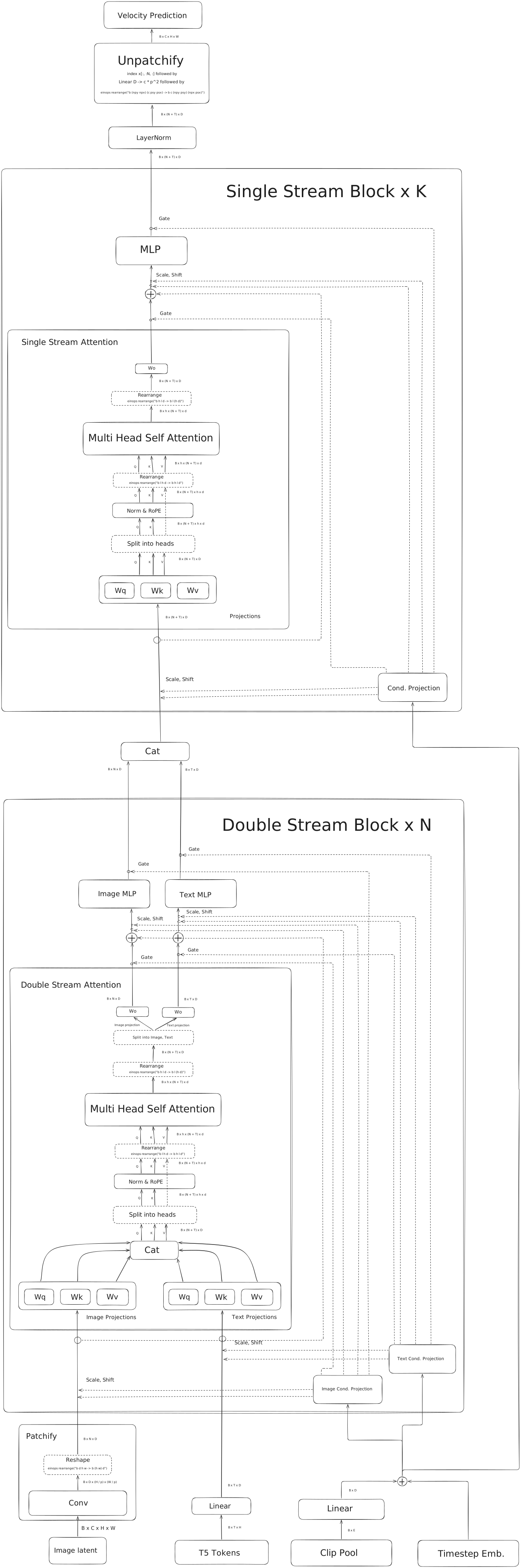
I originally tried using cross-attention instead of the double stream block, where image token queries attend to text keys. This worked, but would have been less effective for classifier-free guidance (CFG) since the attention would have to be skipped entirely for unconditional training, so I decided to switch to a Flux/MM-DiT-style double stream block (fig. 2b) instead later on.

As a little test, once the DiT architecture was implmented, I decided to overfit it on a single image. The model was able to learn and recreate the image, but just barely. It took nearly 10,000 steps and the loss kept plateauing. I was clearly doing something spectacularly wrong.

A bit of digging later, I found that image models (at least the underlying DiTs) don’t operate on actual images. Having a transformer take in raw pixels as an input is very, very costly. Even if you were to use $256 \times 256$ images with a standard patch size of 2, you would end up with a sequence length of $\frac{256^2}{2^2} = 16384$ which is generally far too much to deal with on average hardware if you don’t use some form of modified attention or an extremly tiny model. So, we operate inside of a VAE’s latent space instead.

VAEs

A VAE (Variational Autoencoder) is a type of autoencoder that tries to minimize reconstruction error while keeping a “smooth” latent space. It consists of an encoder model $q_\phi(z \vert x)$ that takes in some input $x$ (eg. an image) and outputs mean ($\mu$) and log variance ($\log \sigma^2$) tensors from which a latent (tensor) or hidden state $z$ is sampled. This latent is then sent through the decoder model $p_\theta(x \vert z)$ that tries to predict the original input $x$. Normally, the latent representation, $z$, is smaller than the input $x$, so the VAE must learn to perform some sort of compression.

\[x \overset{q_\phi(z|x)}{\longrightarrow} z \overset{p_\theta(x|z)}{\longrightarrow} \hat{x}\]

For me, the hardest part about VAEs to understand was the sampling. It seems kind of weird to have a model that doesn’t have full control over its outputs. In VAEs, the latent is literally just noise that was sampled with some given variances and means.

mean, logvar = encoder(x)
z = sample_noise(mean, logvar.exp())
reconstruction = decoder(z)

However, it is important to note that mean and logvar are not scalar values. If $z \in \mathbb{R}^d$, then $\mu, \log \sigma^2$ (mean, logvar) are $\in \mathbb{R}^d$ as well.

This means each value in the latent tensor is sampled from a distribution with given $\mu_i, \log \sigma^2_i$ from the encoder. So, if the model wanted to, it could set all the variances to near zero and have $z \approx \mu$. This is because (somewhat obviously)

\[x \sim \mathcal{N}(\mu, 0) \implies x = \mu\]

So why not just do that? The model could learn to drive its output bias for logvar down to negative infinity ($\sigma^2 \rightarrow 0$) and take complete control over the latent, getting rid of the pesky noise from sampling and turning itself essentially into a “normal” autoencoder.

One of the goals of VAEs is to have a smooth latent space, so that a small change in the latent will still give an output that could reasonably be within the data distribution.

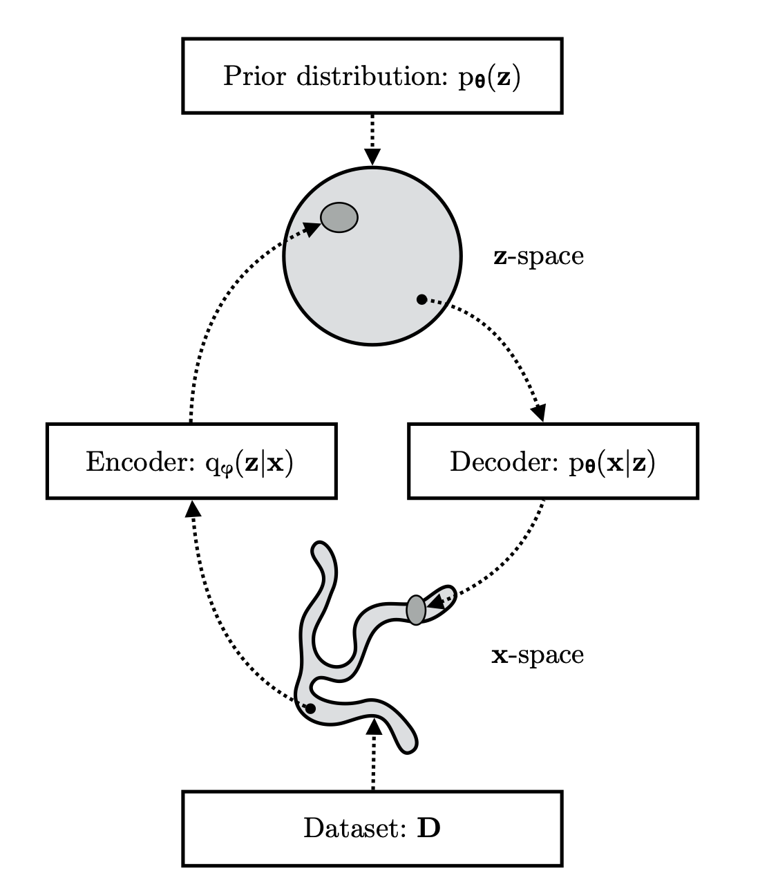From https://arxiv.org/abs/1906.02691, Fig. 2.1

The authors enforce this by adding a KL-divergence term to the loss.

A normal reconstruction loss would be:

\[\mathcal{L}_\text{recon} = \frac{1}{N} \sum_{i=1}^{N} ||x_i - \hat{x}_i||_2^2; \hspace{1cm} \hat{x} \sim p_\theta(x|z), z \sim q_\phi(z|x)\]

In order to keep the latent space from being too sensitive to small changes, the model is penalized for having a latent distribution different from a standard normal distribution $N(0, I)$ with the KL divergence loss term:

\[\mathcal{L}_{KL} = - \frac{1}{2} \sum \left[1 + \log \sigma^2 - \mu^2 - \exp (\log \sigma^2)\right]\]

In practice this is normally weighted by a small amount, like $10^{-4}$. Otherwise, the VAE prioritizes the latent space so much that it is almost entirely unable to learn to reconstruct images.

So, we end up with

\[\mathcal{L}_\text{total} = \mathcal{L}_\text{recon} + \lambda \mathcal{L}_{KL}\]

Where $\lambda$ is the KL loss weight.

But there is a problem. When we try to find the gradients for the encoder, we get stuck.

Since we cannot backpropagate through $z \sim \mathcal{N}(\mu, \sigma^ 2I)$ (how do you take the derivative of a random value with respect to the mean and variance? What is $\frac{\partial z}{\partial \mu}$?), we can’t easily get the gradients. Because of this, we have to use the reparameterization trick.

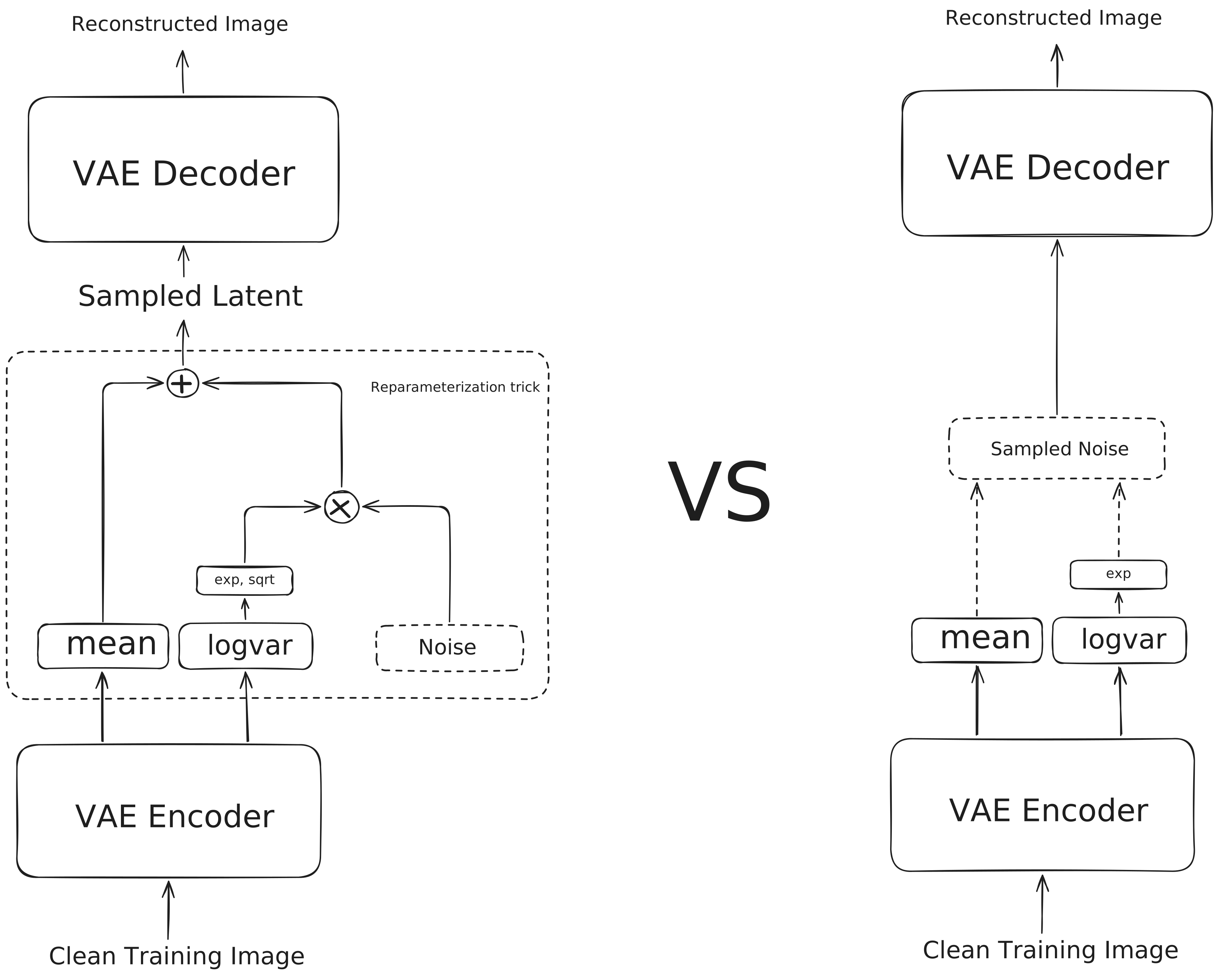Reparameterization trick. Instead of sampling $z \sim \mathcal{N}(\mu, \sigma^2I)$, we sample $\epsilon \sim \mathcal{N}(0, I)$ and let $z = \sigma * \epsilon + \mu$.

The reparameterization trick is simple but clever. Normally, as before, we would do something like:

mean, logvar = encoder(x)
latent = sample_noise(mu, logvar.exp()) # cannot backward through. encoder gets no grad!
reconstruction = decoder(latent)

Which is bad because sample_noise is not differentiable.

To solve this, we sample $\epsilon \sim \mathcal{N}(0, I)$. Then,

\[z = \sigma * \epsilon + \mu\]

This is basically the same thing as sampling $z$ directly. This can easily be differentiated since $z$ is now truly a function of $\mu$ and $\sigma$, also recalling that $\mu = \mu(x; \phi), \sigma = \sigma(x; \phi)$. Now we can do backprop!

mean, logvar = encoder(x)
noise = torch.randn_like(mean) # N(0, I)
latent = (logvar.exp() ** 0.5) * noise + mean # now latent is a function of logvar & mean!
reconstruction = decoder(latent)

For a much better explanation of VAEs, I recommend this paper by the original VAE author. Apparently bro also invented the Adam optimizer. Very much the goat.

---

Traditionally, diffusion model training is done with a pretrained VAE. Images are fed into the encoder, which produces a latent. The latent is then corrupted as an image would be in flow matching. This corrupted image is sent to the DiT which predicts the velocity $z - \epsilon$. At inference, generation starts with random Gaussian noise, which is repeatedly fed into the model and updated as

\[\hat{z}_{t+1} = \hat{z} + \Delta t \cdot v_\theta(\hat{z}_t)\]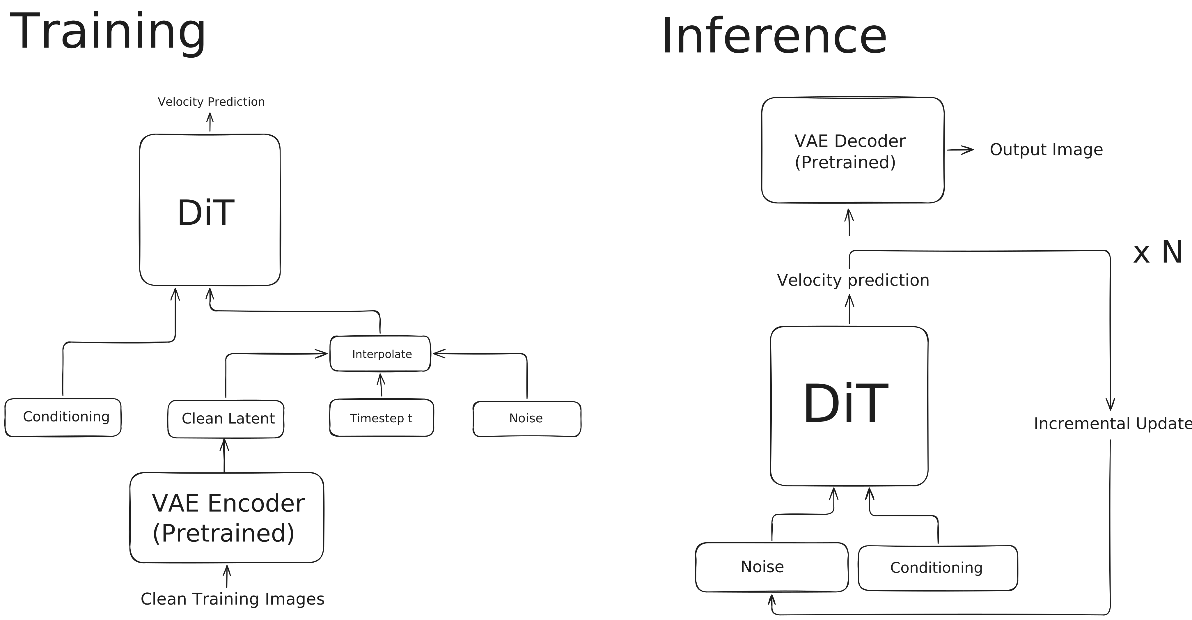

Okay, cool. Instead of doing flow matching on images, we have the VAE encode the images first and do flow matching on the latent. This dramatically reduces the sequence length sent to the DiT because the VAE is doing significant spatial compression when it generates the latent.

This is great, but it’s a little too easy for my tastes. It simply wouldn’t involve enough suffering.

REPA-E

What if I told you there was a magical way to speed up diffusion model training by 45x? Just look at this graph.

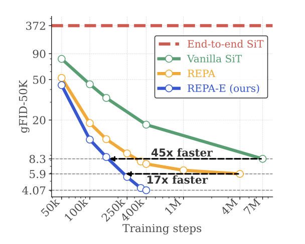Graph taken from https://arxiv.org/abs/2504.10483, Fig. 1d

REPA-E proposes to train the diffusion/flow matching model and VAE at the same time, while using a pretrained encoder model to speed up and stabilize training.

During training, the VAE encoder encodes images as normal into a sampled latent (with reparamerization trick). One copy of the latent is sent to the VAE decoder, and similarity losses are calculated with the input image (along with KL divergence).

Another copy is sent through a BatchNorm layer before being detached, corrupted and sent to the DiT. Without the detach, the VAE encoder would recieve gradients from the diffusion loss, causing it to learn a simplified latent representation in order to make the diffusion process easier, rather than learning to reconstruct images well. The DiT then does velocity prediction on the normalized, corrupted latent (with additional text inputs).

However, the hidden state from one of the DiT layers is kept for later. The image is also sent to a pretrained encoder model, such as DINOv3, which outputs a latent representation. The DiT hidden state is sent through a projection layer (a conv, as in iREPA) and then compared with the pretrained encoder latent using a cosine similarity loss. This incentivizes the model to learn a meaningful and structured representation, speeding up training by taking advantage of the pretrained encoder.

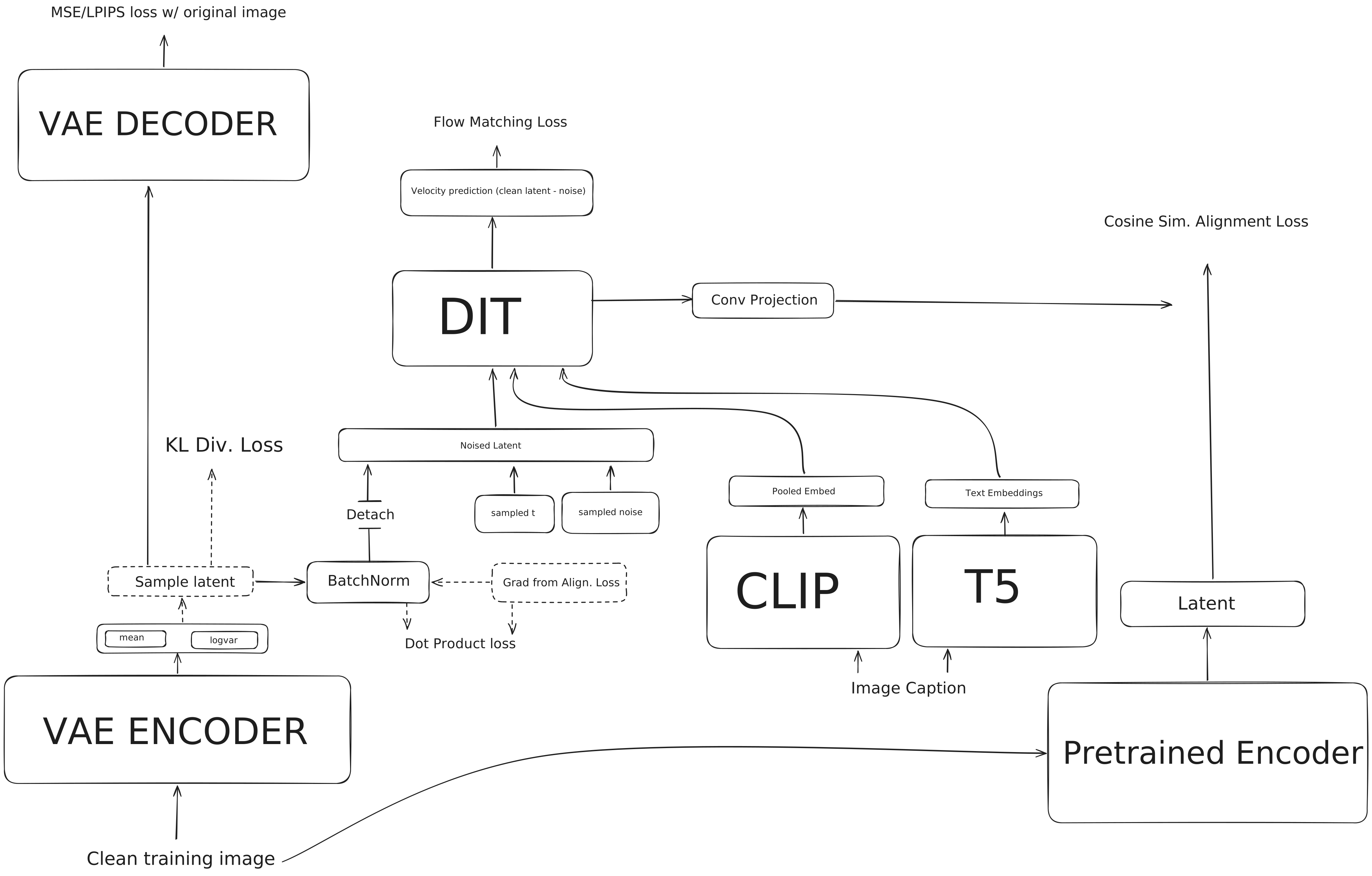Diagram of the REPA-E training setup I used

The gradients from the alignment loss also flow into the encoder model. The latent we used as an input to the DiT was detached to prevent the diffusion loss from having an impact, so it might seem difficult to get gradients for the encoder without running the DiT once again on a non-detached latent.

And running the DiT twice seems to be pretty much what the authors did (lines 372-424). However, that wasn’t good enough for me. Without having seen the source code, I decided to ask Gemini if the model needed to be run twice, and it suggested doing something like the following:

grad_latent_repa = torch.autograd.grad(loss_alignment, latent_detached, retain_graph=True)[0]
loss_encoder_repa = (latent * grad_latent_repa.detach()).sum() # this gives latent the grad calculated with only one forward
loss_encoder_repa.backward()

Which I did, and it seemed to work fine.

REPA-E also uses LPIPS loss for the VAE. LPIPS is a proposed solution to the blurriness caused by training with MSE as an objective. Since MSE is done on a per-pixel basis, a model will be severely punished if, for example, it outputs a nearly-correct image shifted one pixel to the right from the objective. The correct pixel values will be there, but they will be in the wrong positions, causing unnecessarily high loss. As a result, the model learns to make blurry images to avoid getting punished too severly by MSE.

LPIPS uses a pretrained vision model and compares the features it outputs for the predicted and target images. Ideally, the pretrained model will not be sensitive to small pixel shifts, and will be more representative of human judgement. For the LPIPS loss in my setup, I just used the library created by the authors.

---

My initial REPA-E implementation was far from correct. For example, I forgot to pass the noised latent into the dit and passed the clean latent instead, effectively having it predict noise.

I spent about a month and a half trying to get the loss to go down as much as possible. The biggest change was patch_size: 8 -> 2, which is what splits the two big groups of runs in the image below.

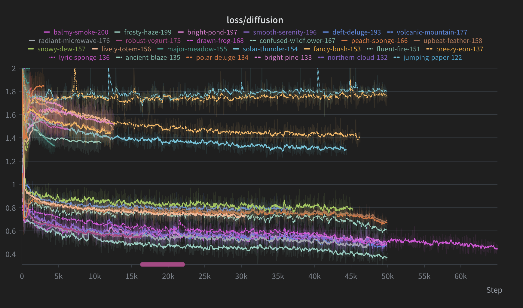
Another important fix I made (although it had no impact on training loss) was to undo the batchnorm transformation at inference time. The DiT operates on normalized latents, not their actual values. So, after the trajectory is simulated in inference, we need to undo the saved BatchNorm normalization.

\[z'_\text{pred} = (z_\text{pred} + \mu_\text{running}) \cdot \sqrt{\sigma^2_\text{running}}\]

Then, $z’_\text{pred}$ is sent to the decoder for the final image.

CFG

Classifier-Free Guidance (CFG) is a method that allows for “low temperature”-like sampling in diffusion models. It involves occasionally dropping conditioning (text inputs) with a certain probability during training, then interpolating between conditioned and unconditioned predictions during sampling with a guidance strength $w$.

While I was looking at CFG, I came across CFG++: Manifold-constrained Classifier Free Guidance for Diffusion Models. This paper proposes a method to solve an issue in regular CFG that causes oversaturated colors and lower image quality (since something about interpolating between predicted noises alone doesn’t work properly).

Finally, as I looked more into CFG++, I noticed that the formulas were all specific to diffusion. This led me to find Rectified-CFG++ for Flow Based Models, which seemed to be exactly what I was looking for.

Their approach is fairly straightforward. Although I don’t really understand the math behind it (what does “bounded tubular neighborhood of the data manifold” mean?), the authors were kind enough to provide a nice algorithm that was easy to implement.

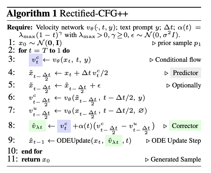The modified CFG sampling algorithm proposed in RF-CFG++

Basically, we just take a half-step in the direction of the velocity predicted by the model with conditioning. From there, we sample both conditional ($v^c_\theta$) and unconditional ($v^u_\theta$) velocities. The difference between the conditional and unconditional velocity is multiplied by some coefficient $\alpha(t)$ and added to the conditional velocity.

My intuition is that $v^c_\theta - v^u_\theta$ gives the vector pointing in the direction that adding the conditioning changes the unconditional veloctity, and adding this vector to the original prediction will make the velocity “even more conditional”.

The hard part about CFG was the modifications I had to make to the training setup. Although they would have been relatively minimial with a normal Flux-style architecture, my original DiT model used cross attention, which wouldn’t really have worked without text for the image tokens to attend to. So, I switched to double stream blocks, which seemed to work much better.

CFG training is described in the paper as something like:

while training:
    x, c = next_data()
    if rand() < p_uncond:
        prediction = model(x)
    else:
        prediction = model(x, c)
    
    # ...

Though this is not the best way to implement it in practice. Having variable inputs is very bad, especially when using torch.compile. I asked GPT if there was a more efficient way to do this, and it said to use masks:

while training:
    x, c = next_data()
    cond_mask = ~(torch.rand(batch_size, 1) < p_uncond)

    prediction = model(x, c, cond_mask)

    # ...

Where cond_mask is used as an attention mask and does not vary in shape. Since I was already using a padding mask for attention, I just multiplied it by cond_mask. However, my smooth monkey brain multiplied the entire attention mask and not just the text part (and also forgot to invert the mask before multplying), so with probability 1 - p_uncond (80% of the time with p_uncond=0.2) the model would just be training on literally nothing. Luckily, it didn’t take me too long to notice and fix this, and the model worked great thereafter.

Additionally, in my setup, I used both normal (T5) and pooled (CLIP) embeddings as conditioning, so in addition to the attention mask, I used torch.where and cond_mask to replace the CLIP conditioning vectors with a learnable null-conditioning vector.

I didn’t see a massive improvement in generation quality from CFG, but the change in architecture did seem to have a significant impact on diffusion loss.

Getting GPUs & DDP

Even with REPA-E, training a diffusion model is still very resource intensive. Far too much for my PC to handle on its own. Thankfully, I am now enrolled at OSU (Go Beavs!), and they have graciously allowed me to (ab)use numerous powerful GPUs via their COE HPC cluster.

In order to take advantage of these GPUs, I had to learn how to use SLURM. Slurm is fairly easy to use, at least in most cases. There are really only 3 commands you need to know how to use:

• srun
• sbatch
• scancel

There is also salloc, but I haven’t really found a use case for it yet.

srun is simple. It lets you allocate some node on a specified partition and gives you an interactive terminal. I find it best to use code tunnel to connect directly to vscode once the node has been allocated.

srun -p dxgh --gres=gpu:2 --constraint=vram80g --mem=32G --cpus-per-task=8 --pty bash

Would allocate me a node in the dgxh partition with two GPUs that have 80g of VRAM each, 32g of memory, and 8 CPU cores.

You can also submit batch jobs with sbatch <your_script.sh>. Just leave comments at the top of the script with #SBATCH --parameter=value to tell slurm what resources to allocate. The rest of the script contains the commands you want to run.

And scancel <job_id> cancels a run.

With this, I was able to start using PyTorch’s DDP. DDP was a bit of a pain to set up at first, but once the boilerplate has been done correctly, it isn’t too difficult. DDP works by spawning a bunch of instances of the training script and setting environment variables like LOCAL_RANK and WORLD_SIZE for each. These can be used with torch.device("cuda:N") to place tensors on the GPU specific to the script.

Trainable modules are wrapped in a DDP object that does communication behind the scenes:

model = DDP(model, device_ids=[local_rank])

A DistributedSampler object is also used for sampling from the dataset so no two ranks use the same data:

dl = torch.utils.data.DataLoader(
    ds,
    batch_size=batch_size,
    pin_memory=True,
    drop_last=True,
    sampler=DistributedSampler(ds) if ddp else None,
    persistent_workers=True,
    num_workers=dataloader_workers_per_rank,
    prefetch_factor=2,
    in_order=False,
)

With all this, I was able to utilize about 200 times the compute I would have gotten on my local GPU, which made the training process feasible.

Results

The final training run I used for my evaluation was 50,000 steps on the Stanford GPIC dataset, with a per-gpu batch size of $32$ on a 4xh100 node for a total batch size with DDP of 128. This run took about $8.5$ hours in total.

Here is a more detailed config:

Parameter	Value
VAE compression	$6 \times$
VAE latent channels	$32$
DiT AdamW lr	$3\times 10^{-4}$ (constant with linear cooldown for last $20\%$)
DiT Muon lr	$1\times 10^{-2}$ (constant with linear cooldown for last $20\%$)
VAE lr (AdamW)	$3\times 10^{-4}$ (constant with linear cooldown for last $20\%$)
Device batch size	$32$
Total batch size	$128$

Given that I have already spent nearly four months on this, in the interest of my own sanity, I have decided not to go down the rabbit hole of evaluating the model’s FID (Fréchet Inception Distance) score and instead will show some qualitative examples.

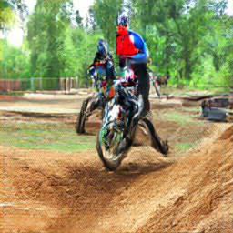A motocross rider in full gear rides an orange dirt bike through muddy terrain. Another rider is visible in the background on a similar trail, with trees and open field surrounding the track.

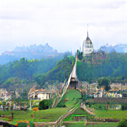A large white church with two tall spires sits at the center of a green village. Surrounding it are houses, trees, and a river in the distance under a cloudy sky.

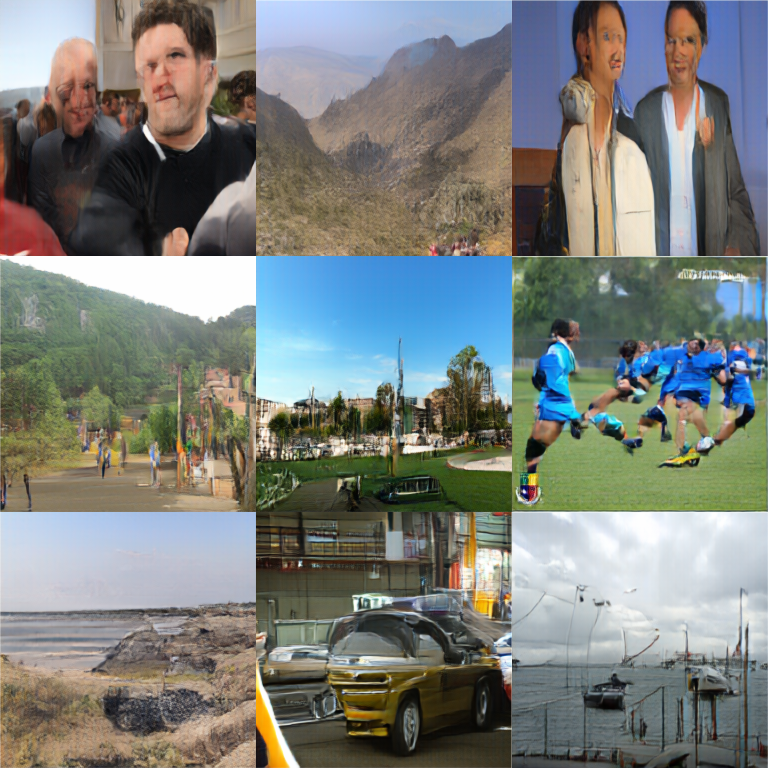Collection of generations by the model

Reflections & What I Learned

I learned a lot while working on this project, and I’m glad that I took the time to make it. One of the most useful things I learned during this time was einops.rearrange().

Einops is an awesome library with multiple features, including einsum and rearrange. Rearrange allows you to specify with symbols how you want to rearrange the elements of a tensor, without having to worry about transpose()/permute()/view()/contiguous(). It also works nicely with torch.compile.

Here’s an example. Suppose you want to write an attention forward pass. Your code is the following:

def forward(x: torch.Tensor) -> torch.Tensor:
    B, T, C = x.size()
    Q = self.rope(norm(self.wq(x).view(B, T, self.n_heads, -1).transpose(1, 2)))
    K = self.rope(norm(self.wk(x).view(B, T, self.n_heads, -1).transpose(1, 2)))
    V = self.wv(x).view(B, T, self.n_heads, -1).transpose(1, 2)

    attn_out = F.scaled_dot_product_attention(Q, K, V, is_causal=True)
    attn_out = attn_out.permute(0, 2, 1, 3).contiguous().view(B, T, C)

    return self.wo(attn_out)

Using einops, it can be rewritten as:

def forward(x: torch.Tensor) -> torch.Tensor:
    Q = self.rope(norm(rearrange(self.wq(x), "b t (h d) -> b h t d", h=self.n_heads)))
    K = self.rope(norm(rearrange(self.wk(x), "b t (h d) -> b h t d", h=self.n_heads)))
    V = rearrange(self.wv(x), "b t (h d) -> b h t d", h=self.n_heads)

    attn_out = rearrange(F.scaled_dot_product_attention(Q, K, V, is_causal=True), "b h t d -> b t (h d)")

    return self.wo(attn_out)

Which, in my opinion, is a lot more readable and easier to work with. I am personally very prone to making mistakes with dimensions, and it seems like einops will make it harder for me to shoot myself in the foot by mixing up my views and transposes.

I also learned to always use pin_memory=True on torch dataloaders. Early on in the project, I was loading images using the builtin huggingface implementation that places data on the specified device. However, this is extremely slow, and it is much faster to just load the data using default huggingface parameters and then load it onto the device using .to(device) with pin_memory=True in the dataloader. This issue was especially prevalent when I started using H100s, as loading the data took longer than running forward and backward on the model by orders of magnitude.

In addition, I found that it is helpful to never use torch.set_default_device(device), as it can hide a lot of mistakes. It is better to just use a torch.device and .to(device) on everything.

Finally, by looking at other codebases to compare to mine, I learned that making things modular/abstracted tends to lead to bad things. Not always, but usually. If your code is nested inside 5 different classes, it will be very difficult to debug. Being lazy is key. Hardcode all your layers if you have to. Do not abstract.

Even something like

class MyVAE(nn.Module):
    def __init__(self, ...):
        super().__init__()

        self.down_layer1 = nn.Conv2d(...)
        self.down_layer2 = nn.Conv2d(...)

        self.act = nn.Tanh()

        self.up_layer1 = nn.ConvTranspose2d(...)
        self.up_layer2 = nn.ConvTranspose2d(...)
        
        # ...

Is probably better than

class MyVAE(nn.Module):
    def __init__(self, ...):
        super().__init__()

        self.encoder = Encoder(...)

        self.act = nn.Tanh()

        self.decoder = Decoder(...)

class Encoder(nn.Module):
    # ...
    self.blocks = nn.ModuleList([EncoderBlock(...) for _ in range(...)])

# ...

I didn’t end up following this rule for this project and abstracted my VAE implementation far too heavily, but I plan to do it in the future to hopefully make my life a little easier.

---

Image generation still seems like a very under-developed field to me. REPA-E was published only around a year ago. The fact that convergence can be sped up by $45 \times$ with a single technique (that was only just discovered) implies to me that Diffusion / Flow Matching might not be the ultimate solution to text-to-image modeling. The whole setup feels cumbersome and bloated, with lots of seemingly unnecessary complexity. Surely, there must be a way to train a decent image model without juggling seven different models at once, and without throwing boatloads of compute into every training run.

Maybe the path forward is just to scale up multimodal transformers. Maybe I should have used an autoregressive model instead of a DiT. Maybe I should have just finetuned z-image to make AI waifus.

I could mope around all day, complaining about how image models still suck. Ultimately, though, I think this was a good experience for me. It’s been very interesting to see how models other than vanilla transformers are implemented and used, and I’ve learned a few helpful tricks along the way.

I am curious to see where this direction of research goes, and hopeful that with LLMs accelerating progress, we will reach a point where powerful image models can be trained even on cheap, local hardware. Although that has yet to happen, learning about image models has at least been a fun project for me.

References

Chandrasegaran, Keshigeyan, et al. “GPIC: A Giant Permissive Image Corpus for Visual Generation.” arXiv.Org, 2026, https://arxiv.org/abs/2605.30341.

Chung, Hyungjin, et al. “CFG++: Manifold-Constrained Classifier Free Guidance for Diffusion Models.” arXiv.Org, 2024, https://arxiv.org/abs/2406.08070.

Esser, Patrick, et al. “Scaling Rectified Flow Transformers for High-Resolution Image Synthesis.” arXiv (Cornell University), Mar. 2024, https://doi.org/10.48550/arxiv.2403.03206.

Ho, Jonathan, and Tim Salimans. “Classifier-Free Diffusion Guidance.” arXiv:2207.12598 [Cs], July 2022, https://arxiv.org/abs/2207.12598.

Kingma, Diederik P., and Max Welling. “An Introduction to Variational Autoencoders.” Foundations and Trends® in Machine Learning, vol. 12, no. 4, 2019, pp. 307–92, https://doi.org/10.1561/2200000056.

Kingma, Diederik P, and Max Welling. “Auto-Encoding Variational Bayes.” arXiv.Org, 20 Dec. 2013, https://arxiv.org/abs/1312.6114.

Leng, Xingjian, et al. “REPA-E: Unlocking VAE for End-to-End Tuning With Latent Diffusion Transformers.” arXiv.Org, 2025, https://arxiv.org/abs/2504.10483.

Lipman, Yaron, et al. “Flow Matching for Generative Modeling.” arXiv.Org, 2022, https://arxiv.org/abs/2210.02747.

Outlier. Diffusion Models From Scratch | Score-Based Generative Models Explained | Math Explained. YouTube, 2024, https://www.youtube.com/watch?v=B4oHJpEJBAA. Video.

———. Flow Matching | Explanation + PyTorch Implementation. YouTube, 2025, https://www.youtube.com/watch?v=7cMzfkWFWhI. Video.

Peebles, William, and Saining Xie. “Scalable Diffusion Models With Transformers.” arXiv.Org, 19 Dec. 2022, https://arxiv.org/abs/2212.09748.

Peter Holderrieth. MIT 6.S184: Flow Matching and Diffusion Models - Lecture 01 - Flow and Diffusion Models (2026). YouTube, 2026, https://www.youtube.com/watch?v=9eJQQVrUUoI&list=PL57nT7tSGAAXwjhDYcxEycx5W7YoSrZyt&index=1. Video.

———. MIT 6.S184: Flow Matching and Diffusion Models - Lecture 02: Flow Matching (2026). YouTube, 2026, https://www.youtube.com/watch?v=PNkMKWW8Khw&list=PL57nT7tSGAAXwjhDYcxEycx5W7YoSrZyt&index=2. Video.

———. MIT 6.S184: Flow Matching and Diffusion Models - Lecture 03A - Score Functions (2026). YouTube, 2026, https://www.youtube.com/watch?v=ngC3QnYSVNM&list=PL57nT7tSGAAXwjhDYcxEycx5W7YoSrZyt&index=3. Video.

Rombach, Robin, et al. “High-Resolution Image Synthesis With Latent Diffusion Models.” arXiv:2112.10752 [Cs], Apr. 2022, https://arxiv.org/abs/2112.10752.

Saini, Shreshth, et al. “Rectified-CFG++ for Flow Based Models.” arXiv.Org, 2025, https://arxiv.org/abs/2510.07631.

Siméoni, Oriane, et al. “DINOv3.” arXiv.Org, 2025, https://arxiv.org/abs/2508.10104.

Singh, Jaskirat, et al. “What Matters for Representation Alignment: Global Information or Spatial Structure?” arXiv.Org, 2025, https://arxiv.org/abs/2512.10794.

Team, Image, et al. Z-Image: An Efficient Image Generation Foundation Model With Single-Stream Diffusion Transformer. 2026, https://arxiv.org/abs/2511.22699.

Zhang, Richard, et al. “The Unreasonable Effectiveness of Deep Features as a Perceptual Metric.” arXiv:1801.03924 [Cs], Apr. 2018, https://arxiv.org/abs/1801.03924.